
This chapter is part of my dissertation. The full thesis is available online as a PDF or can be read chapter by chapter on this website.
Basics of cardiac electrophysiology
The vital mechanical contraction of the heart is driven by electrical waves that travel through the heart muscle tissue—the myocardium. In sinus rhythm—the normal heart rhythm—the heart activates in a well-choreographed sequence to pump blood effectively to the organs: The sinoatrial node in the right atrium acts as the pacemaker of the heart emitting an electrical pulse. The pulse then travels to the left atrium via Bachmann’s bundle, such that both atria contract at the same time. After the pulse reaches the atrioventricular node, it travels through the bundle of His and the Purkinje fibres to and through the ventricular wall, causing the ventricles to contract after the atria (Schiebler, 2005; Zipes & Jalife, 2014). Photographs of an anatomical model of the human heart can be found in Fig. 1.
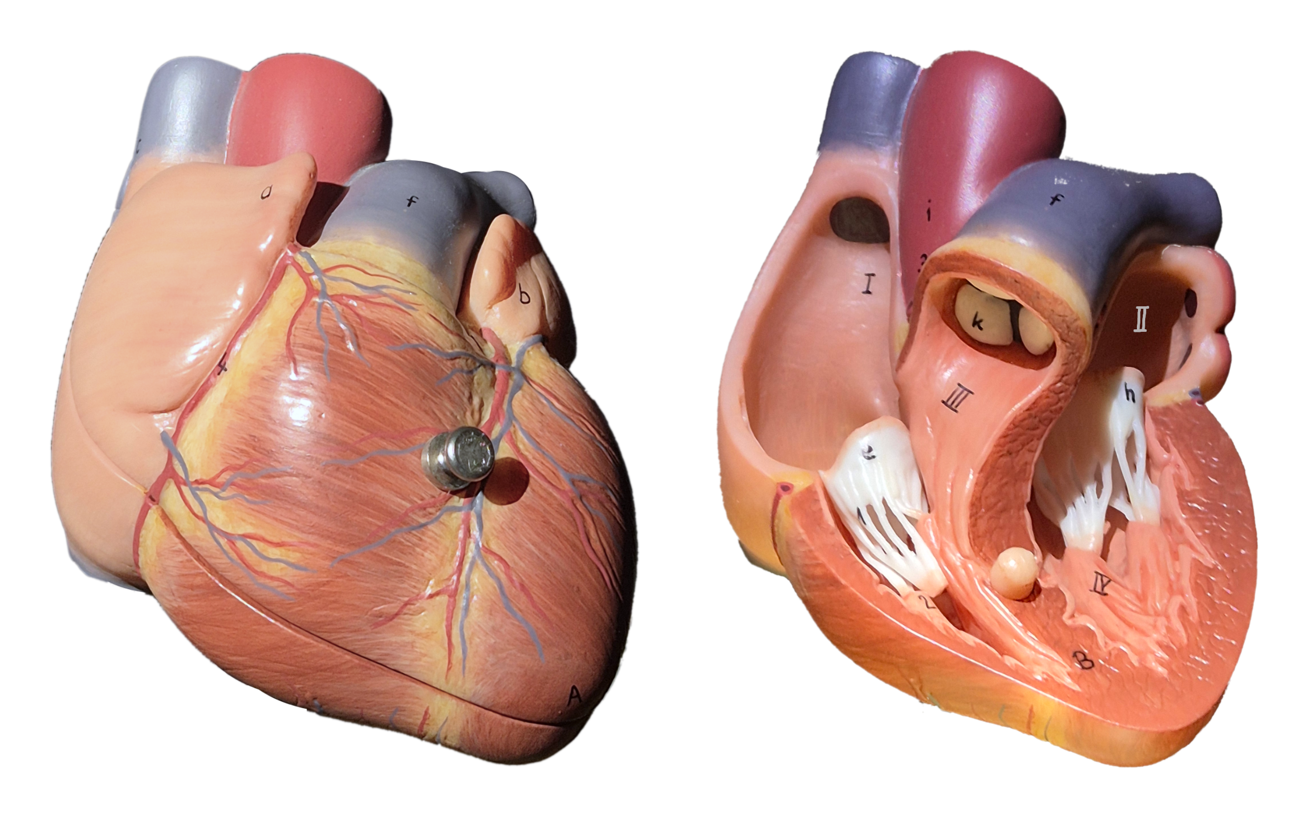
Figure 1: Anterior view of the human heart in an anatomical model. The organ has four chambers: the smaller right (I) and left atria (II) superior of the larger right (III) and left ventricles (IV). Electrical waves coordinate its contraction pumping blood to the organs. Blood-flow is regulated by the opening and closing of valves between the chambers.
Arrhythmias are deviations from this normal heart rhythm. An abnormally low heart rate is called bradycardia1, while an abnormally high heart rate is called tachycardia2. Ventricular tachycardia (VT) is associated with a high risk of sudden cardiac death and is caused by re-entrant circuits in the ventricles, i.e., electrical waves that circulate in the ventricles repeatedly exciting them too early. It can evolve into ventricular fibrillation (VF), which is chaotic electrical activity in the ventricles leading to severely reduced pumping capacity of the heart and sudden cardiac death if not treated immediately with a defibrillator. Atrial fibrillation (AF) is the most common arrhythmia and is not immediately life-threatening, but it can lead to stroke and heart failure if not treated properly (Zipes & Jalife, 2014).
The field of cardiac electrophysiology studies how electrical waves propagate through the heart and how they cause arrhythmias. It is a field that operates on a variety of different levels: from the patient, to the organ, tissue, cell, and subcellular level. The field is highly interdisciplinary, combining knowledge from medicine, biology, chemistry, physics, mathematics, computer science, and engineering. The goal is to not just understand and diagnose the electrical activation patterns, but also to control them to ensure the proper working of each patient’s heart.
In recent years, efforts have been made to create personalised computational models of the heart, so-called cardiac digital twins, which could be used to test and optimise treatment strategies for individual patients (Bhagirath et al., 2024; Costabal et al., 2020; Gillette et al., 2021; Koopsen et al., 2024; Martin et al., 2022; Niederer et al., 2019; Shahi et al., 2022; Trayanova et al., 2020). Machine learning based approaches, for instance, utilising the data from wearable sensors (Chen et al., 2025) and other biomedical applications such as optoelectronics for cardioversion (Portero et al., 2024) show promise to impove the diagnosis and treatment of cardiac arrhythmias and their causes in the coming years. I have contributed to the concept of cardiac digital twins in a variety of ways through scientific articles, some of which are included in this dissertation:
- the development of numerical software to simulate the electrical activity of the heart, see chapter 2 (Kabus, Cloet, et al., 2024),
- the detection of re-entrant circuits in the heart as phase defects, see chapter 3 (Kabus et al., 2022),
- the description of arrhythmia formation via quasiparticles in Feynman-like diagrams, see chapter 4 (Arno et al., 2024a), and
- the creation of data-driven models for cardiac electrophysiology directly from optical voltage mapping data, see chapter 5 (Kabus, De Coster, et al., 2024).
The remainder of this chapter provides background knowledge that is helpful to understand the work presented in the published articles. It begins with a brief overview of cardiac action potentials and central quantities used to describe them. We then discuss the cell cultures and experiments that were conducted to obtain the data used for the creation of the computational models, and how these data are processed. Next, an overview of conventional in-silico models of cardiac electrophysiology is given, followed by an introduction into phase mapping. The introductory chapter concludes with the basics of machine learning on which the data-driven models are based.
Propagation of action potential waves
Excitation waves propagate by neighbouring cells activating each other. Each heart muscle cell—cardiac myocyte—activates and deactivates in a repeating cycle: the action potential. The activation, also known as depolarisation, is much quicker than the deactivation, the repolarisation. The cell’s transmembrane voltage $u$—in units of —is the difference in electrical potential between the inside and the outside of the cell; it is one of the central quantities in the field of cardiac electrophysiology. During the action potential of a single cell, the transmembrane voltage first increases from a resting potential of about to a peak of about exact values vary between cell types. This is called the upstroke of the action potential. After the peak, the voltage remains roughly constant for to the plateau phase, before it decreases back to the resting voltage (Zipes & Jalife, 2014).
We call the time at which $u$ rises above a threshold, the local activation time (LAT); and when it falls below threshold, the local deactivation time (LDT). The time between a cell’s activation and deactivation is called the action potential duration (APD): $$ \text{APD} = \text{LDT} - \text{LAT} \qquad{(1)}$$ Analogously, we call the time between deactivation and activation the diastolic interval (DI): $$ \text{DI} = \text{LAT} - \text{LDT} \qquad{(2)}$$ The cycle length (CL) is the time between two subsequent activations of a cell: $$ \text{CL} = \text{LAT}_2 - \text{LAT}_1 \qquad{(3)}$$ Note that these quantities depend on the chosen threshold. For example, when measured at of the upstroke, the APD is more precisely referred to as APD30 .
Another central quantity is the conduction velocity (CV), which is the speed at which the excitation wave travels through the tissue. It is usually measured as the average speed of the sharp wave front between two points in space: $$ \text{CV} = \frac{\Delta x}{\Delta t} \qquad{(4)}$$ where $\Delta x$ is the distance between the two points and $\Delta t$ is the time it takes for the wave front to travel this distance. This definition is prone to errors when the points are not well-aligned with the direction of wave propagation. Also, as it is averaged, it does not capture local variations in CV. More rigorous definitions exist, for instance, by taking the infinitesimal limit of the above equation and the length of the velocity vector ${{\bm{{v}}}} \in \mathbb R^{D}$, where $D$ is the number of spatial dimensions: $$ \text{CV} = {{\left\lVert {{\bm{{v}}}} \right\rVert}} \qquad{(5)}$$
In Fig. 2, typical action potentials of an atrial model are shown for four pulses in a cable simulation as functions of space and time. In the space-time plot in panel C, the CV is measured as the slope of the wave front. Depending on the timing of the pulses, the APD and CV varies. The fourth pulse is blocked, i.e., it does not propagate through the cable.

Figure 2: Atrial action potentials in a cable simulation. These data were obtained using a numerical simulation of the model by Courtemanche et al. (1998), as will be introduced in section 2.3. A. Subsequent action potentials have different APD30 depending on the previous DI, i.e., timing. B. The excitation wave travels through the cable. C. In a space-time plot of the activation pattern, the CV can be measured as the slope $\Delta x / \Delta t$ of the wave front. In this view, it can also easily be seen that the fourth pulse is blocked.
APD and CV depend on the so-called restitution characteristics which vary between different cell types. Restitution curves are plots of APD or CV against the DI or CL, an example of these curves is shown in Fig. 5.7.
As it has such a big impact on the action potential, the timing of the stimuli is another important aspect of cardiac electrophysiology. The so-called stimulus protocol is the sequence of the timings and locations of the stimuli, usually applied using an electrode. Common protocols are S1S2 where the tissue is re-excited just behind a part of the wave back of a first wave, or burst pacing where several stimuli are applied at the same location in quick succession. Due to inhomogeneities in the tissue, this might lead to re-entry—repeated excitation, which will be discussed below. In stochastic burst pacing (SBP), stimuli at the same electrode location are applied at random intervals to record the response of the tissue to a large variety of timings to get a more complete picture of the cells’ behaviour in unusual settings (Kabus, De Coster, et al., 2024).
A model cell line of human atrial myocytes
To study the electrical properties of cardiomyocytes, it is common to use model cells that can be relatively easily obtained, cultured, and manipulated in the laboratory. There is a wide variety of cells in use, for example neonatal rat ventricular myocytes (NRVMs) (Majumder et al., 2016), or pluripotent stem cell-derived cardiomyocytes (PSC-CMs) (Karakikes et al., 2015).
At Leiden University Medical Center, a new cell line was recently developed that was derived from human fetal atrial tissue which was conditionally immortalised using a lentiviral vector-based system. These so-called human immortalised atrial myocytes (hiAMs) are more representative of human atrial myocytes than other cells enabling their use in a wide range of experiments with cells (Harlaar et al., 2022):
hiAMs are monoclonal, meaning that they are derived from a single cell and are hence genetically identical. This leads to a high consistency in phenotypic properties of the cells, such as their CV and APD. They also posses superior electrophysiological properties compered to human embryonic stem cell-derived atrial myocytes (hESC-AMs) or human induced pluripotent stem cell-derived atrial myocytes (hiPSC-AMs). Observed CVs of hiAMs are around with APD80 of compared to at similar APDs for hESC-AMs (Harlaar et al., 2022).
hiAMs can be expanded almost indefinitely as de-differentiated cells in the presence of the inducing agent doxycycline, and upon its removal, they re-differentiate into functional cardiomyocytes. This allows for the creation of large quantities of cells for experiments, such as the creation of monolayers—one-cell-thick layers grown on a flat surface. As the cells are randomly oriented in the monolayer, the resulting two-dimensional and approximately homogeneous and isotropic tissue can be used to study action potential propagation and re-entry in a controlled way. One use of these monolayers is to study the effects of pro- or anti-arrhythmic drugs on the electrical properties (Harlaar et al., 2022).
A visual outline of the creation of hiAMs is given in figure 1 of the article introducing the cell line (Harlaar et al., 2022): After the cells are isolated from a human fetus, they are transduced with a lentiviral vector encoding the recombinant simian virus 40 large T (SV40LT) antigen under the control of a doxycycline-inducible promoter. The effect of SV40LT on the cells is that they continuously divide. Cell clones are filtered based on selection criteria, such as the ability to proliferate in a doxycycline-dependant manner and to undergo cardiomyogenic differentiation into excitable and contractile cells. The selected cells now have the ability to proliferate in the presence of doxycycline and to differentiate into functional atrial myocytes upon its removal, i.e., without SV40LT expression (Harlaar et al., 2022).
The hiAM cell lines are a promising new tool for studying the electrical properties of the human atria. In chapter 5, optical voltage mapping of focal waves in hiAM monolayers was used as an in-vitro data set to train a data-driven in-silico model. The spiral waves predicted by that model were compared to spiral waves in hiAM monolayers (Kabus, De Coster, et al., 2024). In the following section, we will present some experiments that are commonly performed to measure the electrophysiological activity of cardiomyocytes, such as patch-clamping and optical mapping, which are relevant for the work in this project.
Common experiments in cardiac electrophysiology
Experiments in the discipline of medicine are often graded on a scale from most-invasive to least-invasive as follows, see also Fig. 3:
- In-vivo experiments are performed on living organisms, usually laboratory animals. This is the most realistic setting, but also the most invasive, expensive, and ethically challenging.
- Ex-vivo experiments are performed on tissue samples or organs extracted from organisms that is artificially kept alive outside of the animal. This still requires animal sacrifice.
- In-vitro experiments are performed “in the glass”—i.e., on isolated cells or tissues that are kept alive in a culture dish. Cell lines are cultured to study the behaviour of (populations of) individual cells.
- In-silico experiments are performed on computers. The term refers to the use of silicon in computer chips. This is naturally the least invasive method, but also the most abstract. In-silico models must be created using in-vivo, ex-vivo, or in-vitro data and validated against them.
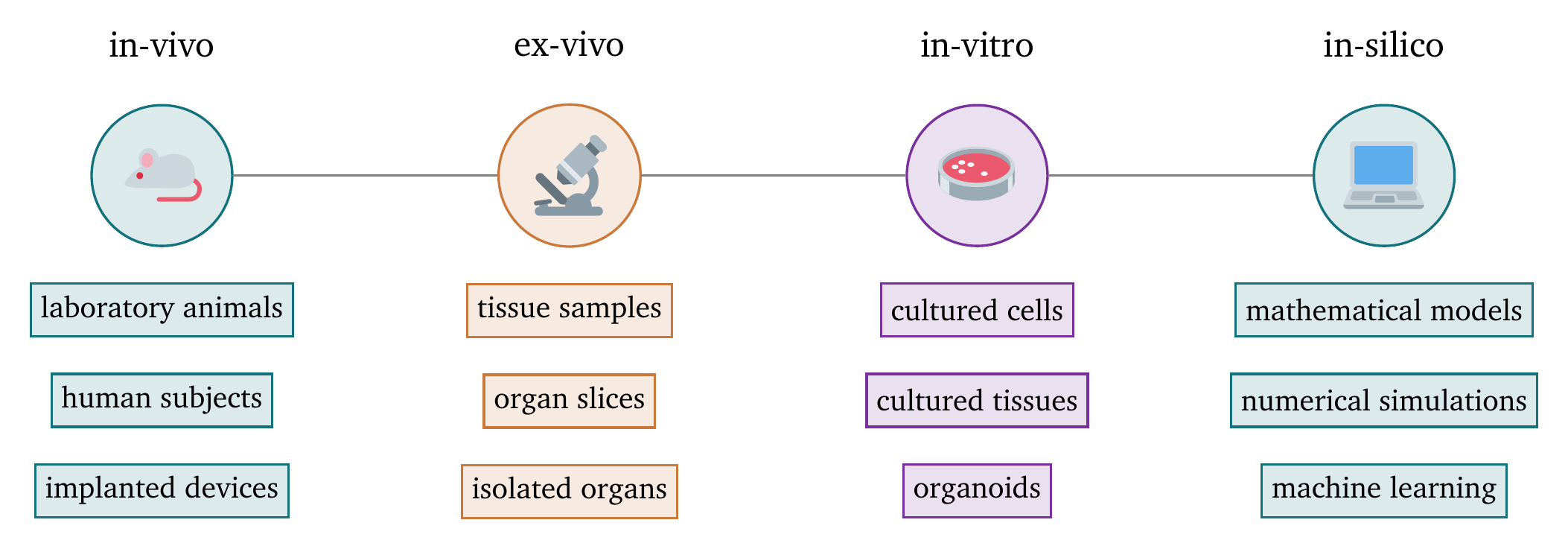
Figure 3: Scale of the invasiveness of medical experiments. The scale ranges from most invasive on the left to least invasive on the right.
In this dissertation, we focus on in-silico experiments motivated by in-vivo, ex-vivo, and in-vitro experiments. In the following sections, we will briefly introduce the types of experiments that are the most relevant for the research presented in this dissertation.
Measurement of single-cell behaviour using patch clamping
Patch clamping is an in-vitro or ex-vivo technique to measure the electrical activity of a single cell. Under a microscope, a glass pipette is carefully attached to the cell membrane. Depending on the quantity that should be measured, the pipette can either leave the cell membrane intact, for instance, to measure the activity of individual ion channels, or penetrate the cell membrane to measure the activity of the entire cell. As the pipette is filled with a solution that conducts electricity, the electrical response of the cell to an applied voltage can be measured (Hill & Stephens, 2021).
Patch clamping was used to measure electrical properties of hiAMs, such as various ionic currents to compare their electrophysiology with that of other cell types. As these cells are an in-vitro model of human atrial myocytes, they should behave similarly to the cells they aim to model. Patch-clamping was therefore mainly used as a tool to validate the hiAMs as a new in-vitro model in the original publication introducing them by Harlaar et al. (2022). This validation justifies the use of hiAMs for future electrophysiological experiments.
Fig. 4 shows how the steady-state current is obtained for a hiAM. A voltage step protocol is applied to stimulate the cell, and the current over time is measured. After an initial transient phase, the current stabilises to the steady-state current. The result of this experiment is a current-voltage curve describing the specific current across the membrane as a function of the applied voltage.
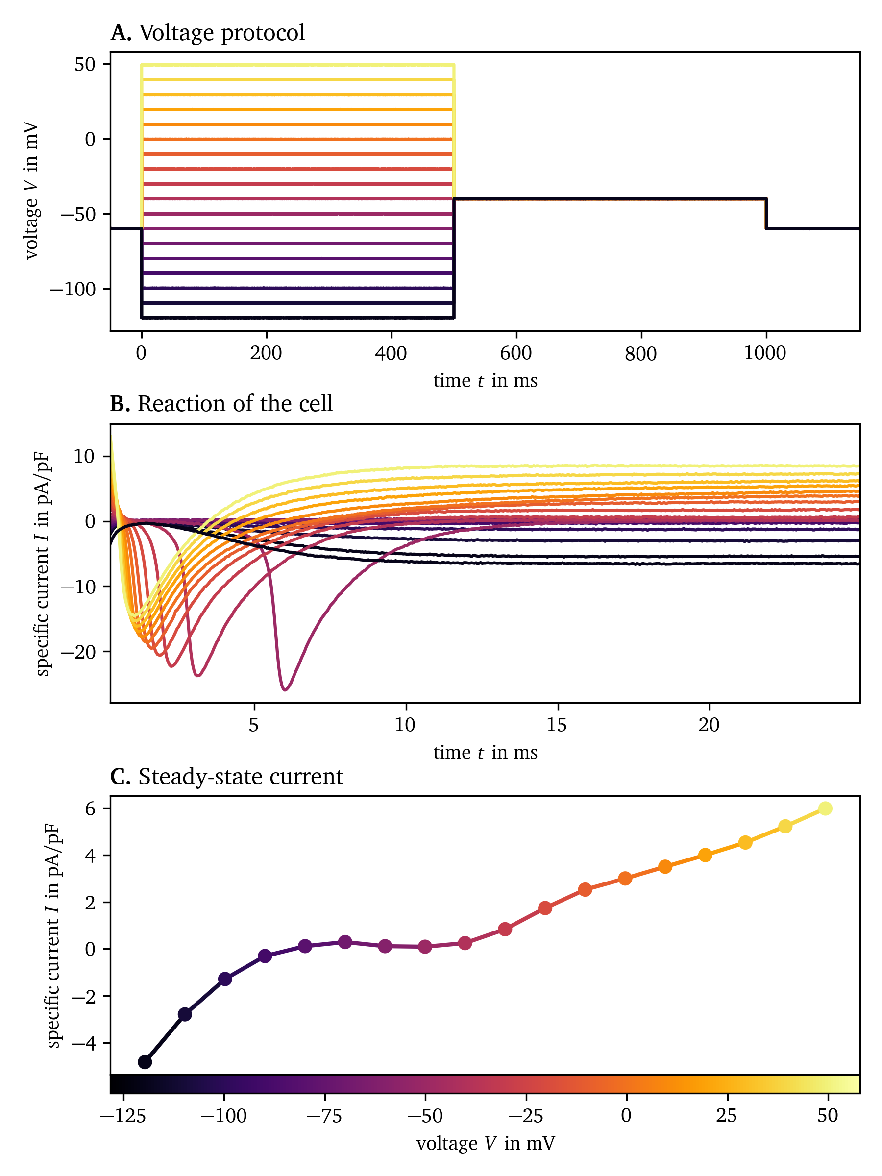
Figure 4: Measurement of the steady-state current of hiAMs using patch clamping. A. The voltage is varied in steps from to and held for . B. The specific current across the membrane is measured for each voltage step. C. Steady-state current as a function of voltage. Experimental data from Harlaar et al. (2022), recorded at Amsterdam Medical Center.
Since the publication of Harlaar et al. (2022), additional patch-clamp experiments have been performed to measure a greater variety of ionic currents in hiAMs. These data are currently being analysed and will be published in a follow-up paper which will introduce a new in-silico electrophysiological model of hiAMs (De Coster et al., in preparation). The in-silico model will follow the classical approach to design a mathematical model of the cells’ electrophysiology to work in the context of the bi- and monodomain description which will be introduced in section 2.
Mapping techniques for tissue-level electrical excitation waves
To study the propagation of excitation waves in cardiac tissue, its electrical activity must be recorded simultaneously at multiple locations. As the electrical activity over space is recorded, this is called mapping. While the transmembrane voltage can not easily be measured directly for mapping, we instead measure by proxy.
On the one hand, electrodes can be used to record the electrical potential in so-called electrograms (EGMs) at different locations, see also section 2.1. The electrodes may be placed on the surface of the tissue or inserted into the tissue. This can be done in-vitro, ex-vivo, or even in-vivo. The electrodes are often arranged in a grid or linear patterns. Catheters with multiple electrodes can be inserted into the heart, such as the PentaRay catheter by Biosense Webster with a 5-star-shaped array of 20 electrodes or the HD Grid catheter by Abbott with a 4x4 grid of electrodes (Berte et al., 2020). Recordings from multiple beats can be combined to create phase maps of recurring patterns of activation, see also section 3.
On the other hand, optical mapping techniques usually record the fluorescence of voltage- or Ca2+ -sensitive dyes (Entcheva & Kay, 2021). A commonly used potentiometric dye is di-4-ANEPPS, which, when it absorbs light in blue to green wavelengths, emits red light whose intensity changes in a way that is approximately proportional to the transmembrane potential (Loew, 1996).
The setup for optical mapping typically consists of the following components: A light source, such as a halogen lamp, whose light may need to be filtered to the desired wavelengths. A dichroic mirror reflects the excitation light to the sample, while allowing the emission light to pass through. An emission filter also blocks the excitation light and only allows the desired, emitted wavelengths to pass through to the camera. The camera and a stimulation mechanism such as an electrode are controlled by a computer. A photograph of a simple optical mapping setup is shown in Fig. 5.
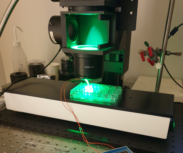
Figure 5: Optical mapping setup with a camera out of frame at the top, green light from the top, lenses for focusing and magnification, and the sample—a 24-well plate. As a simple mechanism for stimulating the tissue, a bipolar electrode is placed in the well. The camera and electrodes are controlled by a computer. To keep the tissue at body temperature, the sample is placed on a heating plate.
Both high temporal and spatial resolution are required for optically mapping the electrical activity of cardiac tissue, fast enough to capture the rapid changes over time and fine enough to capture the details of wave propagation through the tissue. The amount of noise is higher at higher resolutions due to less photons being collected per pixel and frame. Frame rates used for the data collected in this work are in the range of 1 to per frame. The spatial resolution is typically around 150 to per pixel, depending on the choice of lenses and camera. For example, the MiCAM05-Ultima camera by SciMedia has a resolution of 100x100 pixels onto which the imaging plane is projected (Harlaar et al., 2022).
As an example of the data that can be recorded with optical mapping, we show in Fig. 6 a sequence of snapshots of the electrical activity in a hiAM monolayer in a 6-well dish. This experiment shows the formation of a figure-of-eight spiral wave under burst pacing. During subsequent pulses, the gap of blocked conduction between the two sides of a wave front builds up to the point where there is enough space for the front to turn in on itself, creating a pair of spirals.
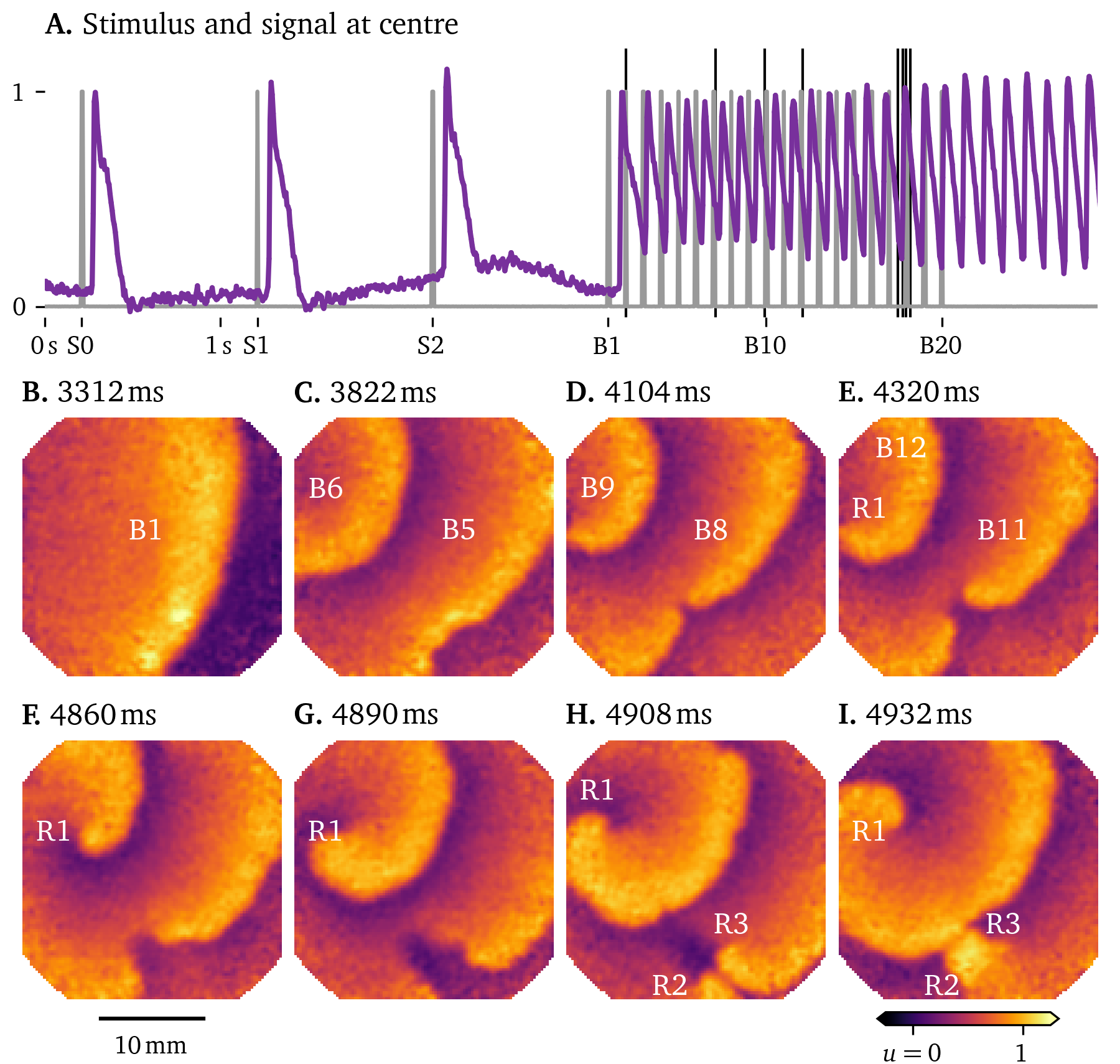
Figure 6: Figure-of-eight spiral formation under burst pacing in hiAM monolayers in a 6-well dish. A. The stimulation protocol in gray consists of three pulses at labelled S1-3, followed by a burst of 20 pulses at , B1-20. These stimuli trigger focal waves emanating from the electrode at the top left in the frame. The response of the central pixel is shown in purple. B.-I. Snapshots of the activity at the times indicated by the thin black lines in A. Frames are chosen at times when an excitation wave crosses a region of interest to show the build-up to figure-of-eight spiral wave formation from pulse to pulse. E. At the top left, a spiral wave forms in sync with the pacing, labelled R1. F.-I. The gap between the two parts of the wave front is so wide, that in the next frames, the wave front can turn around and merge with the next wave front, forming a figure-of-eight spiral wave. H. The two spirals in the figure-of-eight spiral wave are labelled R2 and R3.
In contrast to single cell measurements, optical mapping can capture the complex patterns of excitation waves in tissue. The data are particularly rich as each pixel may have a different time series of excitation and average cell properties, providing a large variability in the data. This variability can be used in the development of data-driven methods to model the electrical activity of cardiac tissue, a main focus of this work.
Processing and analysis of mapping data
Especially at higher resolutions, optical mapping recordings can be so noisy and obscured by other artefacts making it difficult to extract useful information from them. To focus on the relevant parts of the data, there are a variety of processing steps that can be applied. It is important to balance the removal of noise with preservation of the signal without distortion.
One of the most used steps in data processing is smoothing which gets its name from making noisy, jagged data smoother. This is typically done by applying an averaging filter to the data: The smoothed value at a given point is the average of the values of the data points in a small neighbourhood around it. A larger neighbourhood will result in smoother data, but the signal will be less clear, i.e., blurred. If the neighbourhood is too small, the noise will not be removed effectively. Smoothing and blurring are, mathematically speaking, the same operation, which is described by the diffusion equation, also known as the heat equation (Eq. 27). Smoothing can also be done in the frequency domain by applying a low-pass filter, for instance via the Fourier transform. Optical mapping data can be smoothed in time and the two spatial dimensions, note however that smoothing in time violates the causality of the data, meaning that the smoothed data at a given time point will depend on future data points.
A way to smoothen data without violating causality is to use an exponential moving average (EMA). The EMA is a recursive filter that gives more weight to recent data points. The EMA of a time series $u(t)$ at time $t$ is defined as (Heckert et al., 2002): $$ s(t) = \alpha \, u(t) + [1-\alpha] \, s(t-\Delta t) \qquad{(6)}$$ where $s(t)$ is the smoothed data, $\alpha$ is the smoothing factor, and $\Delta t$ is the time step. The EMA gets its name from the fact that the weight of the contribution of each data point to the smoothed value decreases exponentially over time. This can be seen if Eq. 6 is rewritten as: $$ \dot s(t) = \tilde\alpha \, u(t) - \tilde\alpha \, s(t) \qquad{(7)}$$ defining $\tilde\alpha = \frac{\alpha}{\Delta t}$. Multiplyling by ${{\mathrm{e}^{\tilde\alpha t}}}$ and integrating yields: $$ s(t) = {{\mathrm{e}^{-\tilde\alpha t}}} \, u(0) + \tilde\alpha \int_0^t {{\mathrm{e}^{\tilde\alpha \, (t' - t)}}} \, u(t') \;\mathrm{d}t' \qquad{(8)}$$ Hence, the EMA really is a weighted average of the previous data points, with exponentially decaying weights. As it can be efficiently implemented using the recursive formula in Eq. 6, the EMA is a popular choice for smoothing data in real-time applications, such as optical mapping.
Statistical data transformation techniques can also be used to improve the quality of the data. It is common to remove the mean along each dimension in the data and rescale to unit variance. This is called whitening (Abu-Mostafa et al., 2012). For instance, in optical mapping data, the recorded intensity at points that are further away from the camera will be lower than those closer to it. After whitening each pixel by dividing by the standard deviation of its signal over time, the data will have the same variance at each point. This can also be useful for comparing data from different experiments.
To be able to compare optical mapping recordings with electrode-based EGM maps, we can calculate approximate monopolar pseudo-EGMs via a convolution: $$ u_\text{EGM}({{\bm{{x}}}}, t) \propto \int_{\heartsuit} \mathrm{d}{{\bm{{x}}}}' \; \frac{ \nabla \cdot {{\bm{{D}}}} \nabla u(t, {{\bm{{x}}}}') }{ {{\left\lVert {{\bm{{x}}}} - {{\bm{{x}}}}' \right\rVert}} } \qquad{(9)}$$ where ${{\bm{{x}}}}$ is the position of the electrode, $\heartsuit$ is the tissue domain, ${{\bm{{D}}}}$ is the diffusion matrix, and $u$ is the signal representing the transmembrane voltage. These monopolar pseudo-EGMs may be converted to bipolar EGMs by subtracting a reference EGM from each pseudo-EGM. The reference EGM can for instance be any one of the EGMs or the average of all pseudo-EGMs. For more details and additional context, see section 2.1 and chapter 2, (Kabus, Cloet, et al., 2024).
Many quantities of interest in cardiac electrophysiology can be simply obtained via thresholding and differences, such as LAT, LDT, APD, DI, and CL (section 1.1). The CV (Eq. 5) is a quantity that is highly sensitive to noise and artefacts in the data. An elegant algorithm to estimate the velocity vector from LAT maps—a scalar field $T({{\bm{{x}}}})$ in space ${{\bm{{x}}}} \in \mathbb R^{D}$—is the method by Bayly et al. (1998). The gradient $\nabla T$ of this field is the “slowness”—a vector pointing in the same direction as ${{\bm{{v}}}}$, but with the inverse value. We can then obtain the velocity vector via the relation: $$ \begin{aligned} {{\bm{{v}}}} &= \frac{\nabla T}{{{\left\lVert \nabla T \right\rVert}}^2} \end{aligned} \qquad{(10)}$$ However, as LAT increases in discrete steps such that neighbouring grid points either have the same LAT or differ by one or more steps, the gradient is not well-defined. To overcome this, the data can either be smoothed or interpolated for instance by fitting a linear function to the data in a small neighbourhood around each grid point, which is the approach by Bayly et al. (1998).
In Fig. 7, the CV is estimated from LAT and LDT maps of a pulse in the same optical voltage mapping recording of a hiAM monolayer as in Fig. 6. Linear functions—planes—are fitted at each grid point to the neighbouring LAT and LDT values. We use this to get a smooth version of the LAT and LDT maps, as well as the CV via the slope of these planes. It can be seen that in the region of interest where the figure-of-eight reentry forms, the CV of both the wave front and back is lower than in the rest of the tissue, while the APD is prolonged.

Figure 7: Estimation of CV for noisy optical mapping data for the same recording as in Fig. 6. A. Parts of three subsequent excitation waves are passing through the tissue, seen here in the optical signal $u$. B. The smoothed LAT map of pulse B5. C. The smoothed LDT map of pulse B5. D. APD of pulse B5, i.e., the difference of LDT and LAT, is prolonged in the circled region of interest. E. CV of the wave front of pulse B5 is lower in the region of interest. F. The same is true for the CV of the wave back at higher variance.
In the course of this PhD project, besides the main contributions of models of the excitation waves—the reaction-diffusion solvers Pigreads and Ithildin (Kabus, Cloet, et al., 2024) and the data-driven model creation pipeline Distephym (Kabus, De Coster, et al., 2024), to be introduced in the following sections—we have developed various companion software packages to process and analyse the data obtained from the aforementioned experiments: mainly patch clamping, optical mapping, and in-silico simulations. These packages, which contain the methods introduced in this section and more, are (1) the Python module for Ithildin (Kabus et al., 2022; Kabus, De Coster, et al., 2024; Kabus, Cloet, et al., 2024), a Python package to process and analyse excitation wave data, originally designed for data from the reaction-diffusion solver Ithildin and (2) Sappho (Kabus, De Coster, et al., 2024), another Python package to process and analyse optical mapping data. Both packages are compatible with each other. Just as the main contributions, these packages are open-source and available on GitLab.
In-silico models of cardiac electrophysiology
A common way to model the electrical activation patterns that control the mechanical contraction of the heart is the reaction-diffusion equation in the monodomain description. It arises from a number of assumptions about the nature of the electric potentials and ion concentrations in the heart muscle tissue. In this section, we will give a derivation of the monodomain equations from first principles. We will also illustrate how to numerically solve them and present typical solutions to the monodomain equations.
Bidomain description—the cell as an electrical circuit
The first assumption we usually make to describe the electrical activity in the heart’s cells is that the ion concentrations and arising potentials are continuous across the tissue, i.e., instead of looking at the microscopic structure of each cell, we instead zoom out to the mesoscopic tissue scale. The motivation for this is that the activating cells locally show similar behaviour overall—neighbouring cells usually fire together (Tung, 1978). With this assumption, we can now define the electric potentials $u_\text{i}(t, {{\bm{{x}}}})$ on the interior of the cell continuum and $u_\text{e}(t, {{\bm{{x}}}})$ on the exterior, in units of ${\mathrm{{m}{V}}}$ (Clayton et al., 2011; Neu & Krassowska, 1993). These potentials are also commonly referred to as the intra-cellular and extra-cellular potentials, respectively.
The sketch in Fig. 8 shows how the interior and exterior are separated by the cell membrane which consists of a lipid bilayer—modelled as a capacitor, and protein structures which regulate the flow of ions across the cell membrane, i.e., the total ion current $I_\text{ion}$ per unit volume in ${\mathrm{{A}{/}{m}^3}}$. The membrane has a capacitance per unit volume of $C=\beta_\text{m} C_\text{m}$ in ${\mathrm{{F}{/}{m}^3}}$, obtained from the product of the specific cell membrane capacitance $C_\text{m}$ in ${\mathrm{{F}{/}{m}{^2}}}$ and the ratio $\beta_\text{m}$ in ${\mathrm{\frac{1}{m}}}$ of the cells’ surface area to their volume (Clayton et al., 2011). The behaviour of the ion channels in the membrane is quite complex and depends not just on the potentials and ion concentrations, but also on whether or not the structures act like an open or closed “gate”, which is encoded in so-called gating variables. The collective behaviour of the ion channels is described by a cell model for cardiac electrophysiology, which was pioneered by Hodgkin & Huxley (1952) and iterated over in the following decades. In section 2.4.3 and section 2.6, we will provide more detail about a variety of different cell models. The total current across the cell membrane is $C\partial_t u + I_\text{ion}$.
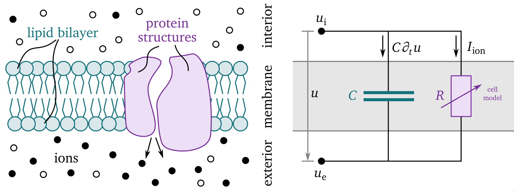
Figure 8: Sketch of the main quantities in the bidomain description. On the left, a close-up view of the cell membrane is depicted which, on the right, is represented by an electical circuit. The membrane separates the cells’ interior from the exterior such that we consider different ion concentrations in each. The lipid bilayer acts like a capacitor $C$ and the protein structures control the ionic currents $I_\text{ion}$, which are here depicted as an adaptive resistor $R$. The difference between the interior and exterior potentials, $u_\text{i}$ and $u_\text{e}$ respectively, is called the transmembrane voltage $u = u_\text{i} - u_\text{e}$. The total current across the cell membrane is $C\partial_t u + I_\text{ion}$. Adapted from Hodgkin & Huxley (1952) and Alberts et al. (2002).
To each of the electric fields on the interior $-\nabla u_\text{i}$ and exterior $-\nabla u_\text{e}$ in units of ${\mathrm{{V}{/}{m}}}$, we can apply Ohm’s law to obtain the current densities $-{{\bm{{\sigma}}}}_\text{i} \nabla u_\text{i}$ and $-{{\bm{{\sigma}}}}_\text{e} \nabla u_\text{e}$ in units of ${\mathrm{{A}{/}{m}{^2}}}$. We denote the conductivity tensors as ${{\bm{{\sigma}}}}_\text{i}$ and ${{\bm{{\sigma}}}}_\text{e}$, for the interior and exterior respectively, in units of ${\mathrm{{S}{/}{m}}} = {\mathrm{\frac{1}{{\Omega}{/}{m}}}}$ (Clayton et al., 2011). These general conductivity tensors enable anisotropic conduction, i.e., current can spread more quickly in some directions, such as along a fibre direction versus across them. More details on the influence of this tensor on the solutions ${{\underline{{u}}}}$ will be provided in section 2.5.
As the current and charge are conserved, the total current across the cell membrane $C\partial_t u + I_\text{ion}$ takes the role of a source term for current densities on the exterior and a sink term on the interior. Therefore, for the divergence of the current densities, we obtain: $$ \nabla\cdot{{\bm{{\sigma}}}}_\text{i} \nabla u_\text{i} = -\nabla\cdot{{\bm{{\sigma}}}}_\text{e} \nabla u_\text{e} = C\partial_t [u_\text{i} - u_\text{e}] + I_\text{ion} \qquad{(11)}$$ By expressing Eq. 11 in terms of the transmembrane voltage $u$ and the extra-cellular potential $u_\text{e}$, we obtain on the domain $\heartsuit\subset\mathbb R^3$ and for duration $T$ in ${\mathrm{{m}{s}}}$: $$ \begin{aligned} C\partial_t u &= \nabla\cdot{{\bm{{\sigma}}}}_\text{i}\nabla[u + u_\text{e}] - I_\text{ion} & \text{on}\,\heartsuit\times[0,T] & \;\;\;\text{(A)} \\ -\nabla\cdot[{{\bm{{\sigma}}}}_\text{i} + {{\bm{{\sigma}}}}_\text{e}] \nabla u_\text{e} &= \nabla\cdot{{\bm{{\sigma}}}}_\text{i} \nabla u & \text{on}\,\heartsuit\times[0,T] & \;\;\;\text{(B)} \\ 0 &= {{\bm{{n}}}} \cdot {{\bm{{\sigma}}}}_\text{i}\nabla[u + u_\text{e}] & \text{on}\,\partial\heartsuit\times[0,T] & \;\;\;\text{(C)} \\ 0 &= {{\bm{{n}}}} \cdot {{\bm{{\sigma}}}}_\text{e}\nabla u_\text{e} & \text{on}\,\partial\heartsuit\times[0,T] & \;\;\;\text{(D)} \\ u &= u_\text{init} & \text{on}\,\heartsuit\times\{0\} & \;\;\;\text{(E)} \\ u_\text{e} &= u_\text{e,init} & \text{on}\,\heartsuit\times\{0\} & \;\;\;\text{(F)} \end{aligned} \qquad{(12)}$$ where, using the normal vector ${{\bm{{n}}}}$ on $\partial\heartsuit$, we have added the boundary condition that no currents may leave the domains, and initial conditions. This is called the bidomain continuum description of activating tissue, due to the assumption of continuous quantities across the two domains outside and inside the cells (Clayton et al., 2011). The boundary conditions for the extra-cellular potential (Eq. 12 D), can further be generalised to couple to the electrical potential around the organ, in the so-called bath (Tung, 1978).
Note that the two main variables in the bidomain equations, the transmembrane voltage $u$ and the extra-cellular potential $u_\text{e}$, are strongly coupled to each other in Eq. 12 B. Their dynamics only differ due to the discrepancy in anisotropy in ${{\bm{{\sigma}}}}_\text{i}$ and ${{\bm{{\sigma}}}}_\text{e}$.
The bidomain equations can be solved with a variety of different numerical methods (Clayton et al., 2011). For instance, a temporal step $t \rightarrow t + \Delta t$ in a naive forward Euler scheme could consist of these tasks:
Calculate the diffusion term: $$ I_\text{i} = \nabla\cdot{{\bm{{\sigma}}}}_\text{i}\nabla[u + u_\text{e}] \qquad{(13)}$$
Update $u$ based on Eq. 12 A: $$ u \leftarrow u + \Delta t [I_\text{i} + I_\text{ion}] \qquad{(14)}$$ respecting the no-flux boundary condition Eq. 12 C.
Calculate the diffusion term: $$ I_u = \nabla\cdot{{\bm{{\sigma}}}}_\text{i} \nabla u \qquad{(15)}$$
Update $u_\text{e}$ by solving the generalised Poisson equation based on Eq. 12 B: $$ \nabla\cdot{{\bm{{\sigma}}}} \nabla u_\text{e} = -I_u \qquad{(16)}$$ with ${{\bm{{\sigma}}}} = {{\bm{{\sigma}}}}_\text{i} + {{\bm{{\sigma}}}}_\text{e}$, respecting the no-flux boundary condition Eq. 12 C.
As it is an elliptic partial differential equation, solving the Poisson equation usually involves implicit solvers which are computationally much more expensive than the solution of the reaction-diffusion equation in the first step, Eq. 12 A.
Monodomain description—a reaction-diffusion system
Another assumption can be made to get to a simpler description of the activation patterns. Assume that the anisotropy of the conduction on the interior and exterior is the same, i.e., let the conductivities be proportional to each other, ${{\bm{{\sigma}}}}_\text{e} := \lambda {{\bm{{\sigma}}}}_\text{i}$ for a dimensionless constant $\lambda > 0$ (Clayton et al., 2011). From Eq. 12, we then obtain: $$ \begin{aligned} &\nabla\cdot{{\bm{{\sigma}}}}_\text{i} \nabla u = -\nabla\cdot[{{\bm{{\sigma}}}}_\text{i} + \lambda {{\bm{{\sigma}}}}_\text{i}] \nabla u_\text{e} = -[1 + \lambda]\nabla\cdot{{\bm{{\sigma}}}}_\text{i} \nabla u_\text{e} \\ \Rightarrow &C\partial_t u = \nabla\cdot{{\bm{{\sigma}}}}_\text{i}\nabla u + \nabla\cdot{{\bm{{\sigma}}}}_\text{i}\nabla u_\text{e} - I_\text{ion} = \nabla\cdot{{\bm{{\sigma}}}}_\text{i}\nabla u - \frac{1}{1+\lambda} \nabla\cdot{{\bm{{\sigma}}}}_\text{i} \nabla u - I_\text{ion} \\ \Rightarrow &\partial_t u = \frac{1}{C} \frac{\lambda}{1+\lambda} \nabla\cdot{{\bm{{\sigma}}}}_\text{i} \nabla u - \frac{I_\text{ion}}{C} \end{aligned} \qquad{(17)}$$
From this, the main monodomain equation follows: $$ \partial_t u = \nabla\cdot{{\bm{{D}}}} \nabla u - \frac{I_\text{ion}}{C} \qquad{(18)}$$ where we have defined the diffusivity tensor $$ {{\bm{{D}}}} := \frac{1}{C} \frac{\lambda}{1+\lambda} {{\bm{{\sigma}}}}_\text{i} \qquad{(19)}$$
The full monodomain description can be obtained by taking the other quantities that influence the ionic currents $I_\text{ion}$ into account. These quantities describe the state of the cells, for instance via ion concentrations and gating variables. These variables are collected in the state variable vector ${{\underline{{u}}}} (t, {{\bm{{x}}}})$ whose first component usually is the transmembrane voltage $u$. Let ${{\underline{{r}}}} ({{\underline{{u}}}})$ be the reaction term whose first component is $r({{\underline{{u}}}}) = - I_\text{ion}/C$ in ${\mathrm{{V}{/}{s}}}$. We can then rewrite Eq. 18 as the reaction-diffusion equation: $$ \partial_t {{\underline{{u}}}} = {{\underline{{P}}}} \nabla \cdot {{\bm{{D}}}} \nabla {{\underline{{u}}}} + {{\underline{{r}}}} ({{\underline{{u}}}}) \qquad{(20)}$$ where the unitless projection matrix ${{\underline{{P}}}}$ encodes whether a variable is to be subjected to the diffusion operator. For most cell models, only the transmembrane voltage is diffused, ${{\underline{{P}}}} = \operatorname{diag}(1, 0, ..., 0)$.
A side note on notation: We use different notation to distinguish vectors and matrices in physical space and state space. Capital letters are used for matrices, ${{\bm{{D}}}}$, ${{\underline{{P}}}}$; while lowercase letters are used for vectors, ${{\bm{{x}}}}$, ${{\underline{{u}}}}$. Boldface symbols are vectors or matrices in physical space, ${{\bm{{x}}}}$, ${{\bm{{D}}}}$; while underlined quantities are vectors or matrices with respect to the state variables, ${{\underline{{u}}}}$, ${{\underline{{P}}}}$. To illustrate this notation, Eq. 20 would read as follows in Einstein sum notation (Kabus, Cloet, et al., 2024): $$ \partial_t u_m(t,{{\bm{{x}}}}) = P_{mm'} \; \partial_{n} D_{nn'}({{\bm{{x}}}}) \; \partial_{n'} u_{m'}(t, {{\bm{{x}}}}) + r_{m}({{\underline{{u}}}};{{\bm{{x}}}}) \qquad{(21)}$$ where $m, m' \in \{1, ..., M\}$ for $M$ state variables and $n, n' \in \{1, 2, 3\}$ the spatial dimensions with $\partial_n = \partial_{x_n}$.
With no-flux boundary and initial conditions, the full monodomain description takes the form of this system of partial differential equations: $$ \begin{aligned} \partial_t {{\underline{{u}}}} &= {{\underline{{P}}}} \nabla \cdot {{\bm{{D}}}} \nabla {{\underline{{u}}}} + {{\underline{{r}}}} ({{\underline{{u}}}}) & \text{on}\,\heartsuit\times[0,T] & \;\;\;\text{(A)} \\ 0 &= {{\bm{{n}}}} \cdot \nabla {{\underline{{u}}}} & \text{on}\,\partial\heartsuit\times[0,T] & \;\;\;\text{(B)} \\ {{\underline{{u}}}} &= {{\underline{{u}}}}_\text{init} & \text{on}\,\heartsuit\times\{0\} & \;\;\;\text{(C)} \end{aligned} \qquad{(22)}$$
In a more general context, the monodomain equations are an example of a reaction-diffusion system, which can be used to describe a wide variety of phenomomena. All kinds of excitation waves can be modelled as reaction-diffusion systems, which, besides muscle tissue and other tissues in the body like coupled neurons (Cannon et al., 2014), includes waves in chemistry (Kapral & Showalter, 1995; Rotermund et al., 1990), or, more abstractly, the spread of epidemics (Arno et al., 2024a; Lechleiter et al., 1991). Even the propagation of a mexican wave in a sports stadium, or the spread of forest fires with subsequent recovery (Fig. 9) can be seen as excitable media.
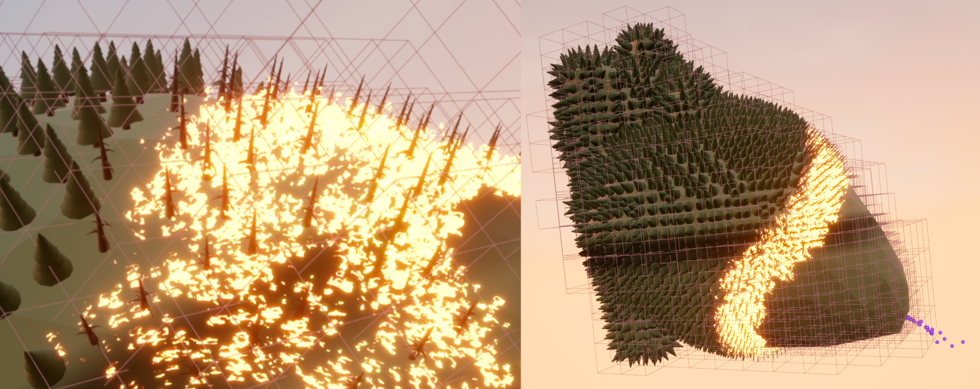
Figure 9: Forest fires as an excitable system can also be modelled by the reaction-diffusion equations (Eq. 22). In the depicted non-scientific simulation, the spread of a forest fire is modelled on a planet in the shape of a human heart to illustrate the similarities between the two phenomena of wildfire spread and cardiac electrical excitation waves. CC-BY 2022 Judith Verdonck, Desmond Kabus et al.; Team HeartKOR at KU Leuven and Digital Arts and Entertainment at Howest.
Numerical solvers of reaction-diffusion problems
To solve the monodomain equations (Eq. 22) numerically, in contrast to the bidomain equations, one now does not need to solve Poisson’s equation. A forward Euler scheme for this is:
Calculate the diffusion term: $$ {{\underline{{d}}}} = {{\underline{{P}}}} \nabla \cdot {{\bm{{D}}}} \nabla {{\underline{{u}}}} \qquad{(23)}$$
Update ${{\underline{{u}}}}$ based on Eq. 22 A: $$ {{\underline{{u}}}} \leftarrow {{\underline{{u}}}} + \Delta t [{{\underline{{d}}}} + {{\underline{{r}}}}] \qquad{(24)}$$ respecting the no-flux boundary condition Eq. 22 B.
While this simpler numerical scheme is an advantage of the monodomain over the bidomain description, the monodomain description has the disadvantage that it is at a higher level of abstraction from the physical reality. Some level of detail necessarily gets lost during abstraction. For instance, one can not exactly recover the intra- and extra-cellular potentials, $u_\text{i}$ and $u_\text{e}$, from the transmembrane voltage $u$.
A variety of finite-differences or -elements software has been published to solve Eq. 22, some of which also have support for solving the bidomain description, Eq. 12, (Africa et al., 2023; Antonioletti et al., 2017; Arens et al., 2018; CARMEN, 2024; Cooper et al., 2020; Finsberg et al., 2023; Niederer et al., 2011; Plank et al., 2021; Rognes et al., 2017). To have control of every aspect of the numerical solution, we have also developed our own reaction-diffusion solvers. By designing every component that goes into the software ourselves, we can optimise the code perfectly for our use cases, such as including tools geared towards cardiac electrophysiology and omitting features that are irrelevant to us. Additionally, we can tweak the code to ideally match available hardware.
The first of our reaction-diffusion solvers is Ithildin (Kabus, Cloet, et al., 2024): It was written in the C++ programming language (ISO, 2023) and utilises parallelisation with OpenMPI (Graham et al., 2006), an open implementation of the message passing interface (MPI), for efficient simulations in 2D and 3D on central processing units (CPUs). It also offers a wide variety of methods for recording additional data during the simulation, such as pseudo-EGMs. Beginning with work by C. Zemlin and O. Bernus and continued development by H. Dierckx from 2009 onwards, in this PhD project, this code was polished, thoroughly improving its code in regards to the numerical methods and user-friendliness. Ithildin was published as a scientific research paper for this PhD project which is reproduced in chapter 2.
A more minimal alternative is the Python-integrated GPU-enabled reaction diffusion solver, or in short Pigreads, which we wrote to be published along with this dissertation. Instead of on CPUs, Pigreads solves the reaction-diffusion equation on graphical processing units (GPUs). While GPUs are, as the name implies, designed for calculations related to computer graphics—such as rendering 3D objects, shaders, or image processing, all of their computational power is opened up in general-purpose computing on GPUs (GPGPU). This paradigm is particularly useful for highly-parallel numerical problems, for instance, where at each of a large number of points, the same equations need to be solved independently from one another. While there are multiple solutions to utilise GPGPU capabilities, for Pigreads, we use the Open Computing Language (OpenCL) (Stone et al., 2010) to enable cross-platform GPU-parallelisation. For instance, on Nvidia GPUs, OpenCL capabilities are provided by the proprietary but highly-optimised Compute Unified Device Architecture (CUDA) (Du et al., 2012; Nickolls et al., 2008). Similar implementations exist for other GPU architectures; there even is a CPU fallback making it possible to run Pigreads on machines without a dedicated GPU. Pigreads is designed to have as little overhead as possible, only solving the reaction-diffusion equations (Eq. 22), without any bells and whistles for maximal performance. Instead, it is relying on a simple interface with the Python programming language via Pybind11 (Jakob et al., 2017; van Rossum et al., 1995). This way, any desired custom feature can easily be implemented in a Python script with numerical and scientific Python (Harris et al., 2020; Virtanen et al., 2020) which then calls the Pigreads module.
Both of our solvers, Ithildin and Pigreads, use central finite differences to implement the spatial derivatives in Eq. 22, such as the diffusion term $\nabla \cdot {{\bm{{D}}}} \nabla u$. In the finite differences method, derivatives are approximated by calculating a weighted sum in a neighbourhood around each point on a grid—the discretisation of the domain $\heartsuit$. For instance, the one-dimensional Laplacian $\partial_x^2 u$ can be calculated as: $$ \partial^2_x u(x) \approx \frac{u(x + \Delta x) - 2 u(x) + u(x - \Delta x)}{\Delta x^2} \qquad{(25)}$$ which is an approximation that is accurate to the second order of the grid spacing $\Delta x > 0$. The weights in this case are $\frac{1}{\Delta x^2}$ for the previous and following grid point, and $\frac{-2}{\Delta x^2}$ for the grid point $x$ to calculate the Laplacian at. Note that these weights need to be adjusted if any of the neighbouring points are outside of the domain. Finite-difference weights numerically discretising the diffusion term $\nabla \cdot {{\bm{{D}}}} \nabla u$ and respecting the no-flux boundary conditions (Eq. 22) also depend on the varying value of ${{\bm{{D}}}}({{\bm{{x}}}})$ over space. The diffusion matrix ${{\bm{{D}}}}$ is usually left constant in time though, such that the weights must be calculated only once at the beginning of the numerical simulation (Clayton et al., 2011).
A final issue to address in the design of finite differences solvers of Eq. 22 using an forward Euler time stepping scheme is the Courant-Friedrichs-Lewy (CFL) numerical stability criterion (Courant et al., 1928): If the time step $\Delta t$ is too large, critical details of the wave propagation in the reaction-diffusion equation might be neglegted leading to an inaccurate or even unstable solution, i.e., $u \rightarrow \infty$. The CFL condition ensures that $\Delta t$ is small enough such that the waves do not travel further than one spatial grid point during each time step. Ithildin automatically sets the time step low enough to satisfy the criterion as follows (Kabus, Cloet, et al., 2024; Li et al., 1994): $$ \Delta t < {{\left[ 2\max{({{\underline{{P}}}})} \sum_{n=1}^{N} \frac{D_{nn}}{\Delta x_n^2} \right]}}^{-1} \qquad{(26)}$$ Therefore, the maximum time step is linked to the chosen grid spacing.
Common solutions of reaction-diffusion problems
The heat equation
The two terms on the right-hand side of Eq. 22 A, encode the two mechanisms enabling the propagation of excitation waves. The diffusion term ${{\underline{{P}}}} \nabla \cdot {{\bm{{D}}}} \nabla {{\underline{{u}}}}$ spatially couples the medium and leads to the spreading of ${{\underline{{u}}}}$. Considering only the diffusion term, i.e., for the trivial model ${{\underline{{r}}}} = 0$, Eq. 22 is reduced to the heat equation: $$ \begin{aligned} \partial_t u &= \nabla \cdot {{\bm{{D}}}} \nabla u & \text{on}\,\heartsuit\times[0,T] & \;\;\;\text{(A)} \\ 0 &= {{\bm{{n}}}} \cdot \nabla u & \text{on}\,\partial\heartsuit\times[0,T] & \;\;\;\text{(B)} \\ u &= u_\text{init} & \text{on}\,\heartsuit\times\{0\} & \;\;\;\text{(C)} \end{aligned} \qquad{(27)}$$ An example of a typical solution $u(t, {{\bm{{x}}}})$ of the heat equation is obtained via numerical simulation using Pigreads and shown in Fig. 10: The sharp right angles of the square-shaped heat distribution $u_\text{init}(x)$ at $t=0$, gradually get smoothed out such that the temperature will eventually equalise in the entire domain for $t\to\infty$. These equations also describe how initially uneven concentrations of chemicals eventually reach a homogeneous steady-state through diffusion, which is why Eq. 27 A is sometimes also called the diffusion equation. This is also the origin of the names of the diffusion term, diffusion operator, etc.

Figure 10: A solution of the heat equation. The heat equation (Eq. 27) describes that an initially uneven distribution of heat gets diffused until a steady-state of homogeneous temperature is reached.
The model by P. Gray & Scott (1983)
The reaction term ${{\underline{{r}}}}$ describes the local reaction at each point of the medium $\heartsuit$. Let there be two variables, ${{\underline{{u}}}} = {{{{\left[ a, b \right]}}}^\mathrm{T}}$, scaled to the interval $[0,1]$, which each describe the concentrations of one of two chemicals $A$ and $B$. One of the models by P. Gray & Scott (1983) describes the chemical reactions: $$ \begin{aligned} A + 2B &\to 3B & \;\;\;\text{(A)} \\ B &\to C & \;\;\;\text{(B)} \end{aligned} \qquad{(28)}$$ for the product $C$. Reactant $A$ is fed into the system at rate $f$, a model parameter; and the parameter $k$ determines how quickly reactant $B$ is removed. $A$ takes the role of an activator whose presence increases the reaction rate, while $B$ inhibits, i.e., slows down the reaction. The model equations then take the form: $$ \begin{aligned} \partial_t a &= D_a \nabla^2 a - a b^2 + f [1 - a] & \;\;\;\text{(A)} \\ \partial_t b &= D_b \nabla^2 b + a b^2 - [f + k] b & \;\;\;\text{(B)} \end{aligned} \qquad{(29)}$$ with diffusivities $D_a = 1$ and $D_b = 0.5$. For various parameters $k$ and $f$, the solutions of Eq. 29 are leopard-like dotted patterns or zebra-like line patterns, or even spiral waves. For example, Fig. 11 illustrates a Pigreads simulation of the model with $k = 0.062$ and $f = 0.055$ starting at a triangular initial distribution of $B$ and constant maximal concentration $a=1$ of reactant $A$. We used a grid spacing of $\Delta x = \Delta y = 1$ and a time step of $\Delta t = 0.1$ in arbitrary spatial and temporal units.
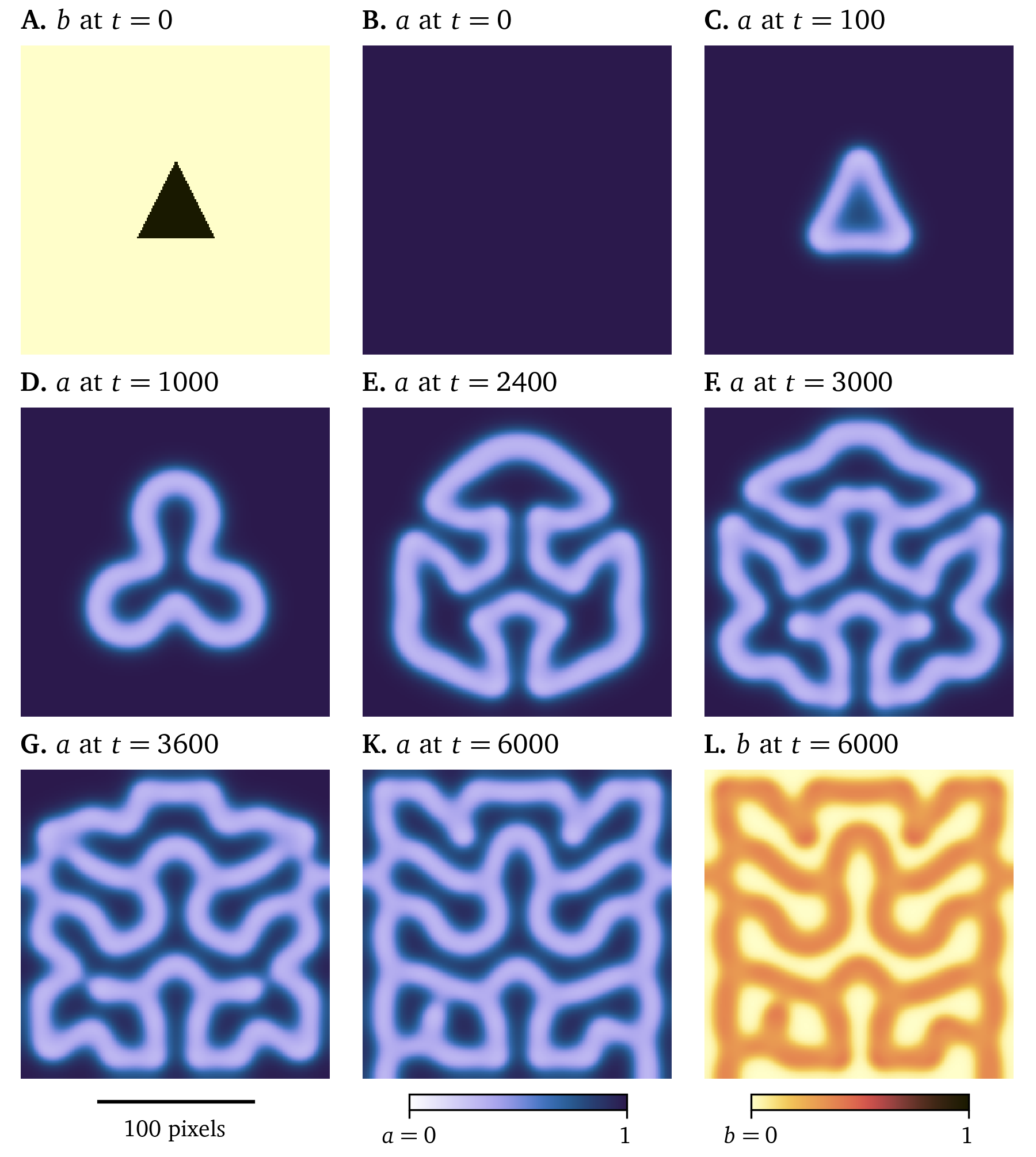
Figure 11: A solution of the model by P. Gray & Scott (1983). Starting from a simple initial condition in chemical $B$, a complex shape develops for parameters $k = 0.062$ and $f = 0.055$, cf. Eq. 29. Arbitrary units in time and space are used, the concentrations $a$ and $b$ are scaled to [0,1].
This example illustrates how the interplay of diffusion and reaction can lead to complex and chaotic behaviour: Slight variations in initial conditions can lead to vastly different outcomes.
Excitation waves in cardiac muscle tissue
Nowadays, there is a large variety of electrophysiological models that describe the excitation waves that can be found in various cells. One of the first and most influential was the model of the giant squid axon by Hodgkin & Huxley (1952), describing the neurons as an electrical circuit, as described in section 2.1, gaining them the 1963 Nobel Prize in Physiology or Medicine (Nobel Prize, 1963).
Most models fit into two categories: phenomenological and detailed ionic models. The detailed models (Courtemanche et al., 1998; Majumder et al., 2016; Paci et al., 2013; ten Tusscher & Panfilov, 2006) aim to describe as many electrophysiological processes inside each cell as possible to provide a full description of their behaviour starting on the single cell level, zooming out to the tissue level. The goal of the phenomenological models is to describe the overall wave dynamics on the tissue level while simplifying microscopic details within the cells. This reduces their computational cost, such that larger scale simulations are possible than with more detailed models. The model by FitzHugh (1961) and Nagumo et al. (1962) can be seen as a two-variable simplification of the four-variable Hodgkin & Huxley (1952) model. The model by Barkley (1991) follows similar design goals, however it was specifically designed to simulate the spiral waves arising in the Belousov-Zhabotinsky reaction. Other early phenomenological models specifically designed for cardiac excitation patterns are the models by Karma (1993); Aliev & Panfilov (1996), Fenton & Karma (1998), and C. Mitchell (2003). The minimal four-variable model by Bueno-Orovio et al. (2008) can be used to emulate other models, such as the ones by ten Tusscher et al. (2004) or Priebe & Beuckelmann (1998).
Using the smoothed version of the Karma model (Byrne et al., 2015; Karma, 1993, 1994; Marcotte & Grigoriev, 2017), we have run a Pigreads simulation on a monolayer, i.e., two-dimensional tissue, approximately in 6-well size ($R = {11~\mathrm{{m}{m}}}$) at a resolution of 200x200 pixels, with homogeneous and isotropic diffusivity $D = {0.03~\mathrm{{mm}^2{/}{m}{s}}}$, with selection matrix $P_u = 1$ and $P_v = 0.05$ for the state variables ${{\underline{{u}}}} = {{{{\left[ u, v \right]}}}^\mathrm{T}}$, using a time step of $\Delta t = 0.025$. In this simulation in Fig. 12, some of the typical electrophysiological behaviour of cardiac myocytes can be observed: The state variable $u$ which represents the transmembrane voltage in arbitrary units, smoothly switches between excited and resting state in waves of excitation that propagate through the medium. The depolarisation at the wave front, the up-stroke, occurs on a quicker time-scale than the repolarisation at the wave back. Between excitation and recovery, the transmembrane voltage stays roughly constant in the so-called plateau phase. This cycle from polarised resting state, over upstroke, plateau, and recovery, back to the resting state is called an action potential. The restitution variable $v$ describes the internal state of the cells, most crucially how recently the waves have been excited. At a high value of this variable $v$, excitation is inhibited, as can be seen at $t={0~\mathrm{{m}{s}}}$ in Fig. 12 A.
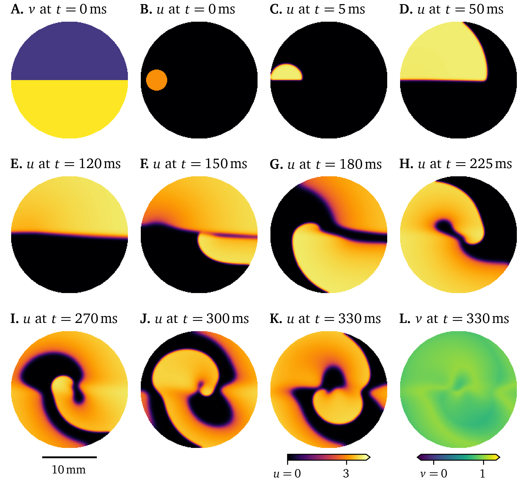
Figure 12: Simulation of the smoothed Karma model in a 6-well monolayer. Due to the initial distribution of the restitution variable, a rotor forms.
In this simulation (Fig. 12), we have chosen initial conditions such that a rotor forms: Due to the high value of $v=1$ in the lower half of the monolayer at $t={0~\mathrm{{m}{s}}}$, the initial stimulus in $u$ only triggers an action potential in the upper half, a conduction block line between the halves forms. Once the tissue recovers, it is again possible to excite the lower half. The wave turns around and follows the conduction block line creating a spiral wave rotor. These re-entrant waves have been identified as one of the mechanisms of tachycardia (R. A. Gray et al., 1995).
Influence of tissue heterogeneity and anisotropy on electrical excitation waves in the heart
An anisotropic diffusivity tensor ${{\bm{{D}}}}$, i.e., one that is not the same in every direction, encodes at which time scale diffusion—and equivalently conduction—takes place in the different directions. Cardiac muscle tissue is structured in fibres that may be further aligned in sheets. The diffusion along the fibres, encoded in diffusivity $D_{\text{f}}$, and within the sheets, $D_{\text{s}}$, is faster than in the normal direction, $D_{\text{n}}$ (Clayton et al., 2011): $$ {{\bm{{D}}}} = D_{\text{f}} {{\bm{{e}}}}_{\text{f}} {{{{\bm{{e}}}}}^\mathrm{T}}_{\text{f}} + D_{\text{s}} {{\bm{{e}}}}_{\text{s}} {{{{\bm{{e}}}}}^\mathrm{T}}_{\text{s}} + D_{\text{n}} {{\bm{{e}}}}_{\text{n}} {{{{\bm{{e}}}}}^\mathrm{T}}_{\text{n}} \qquad{(30)}$$ for the orthonormal basis vectors ${{\bm{{e}}}}_\text{f,s,n}$ along the fibres, within the sheet, and normal to the sheets, and ${{\bm{{a}}}} {{{{\bm{{b}}}}}^\mathrm{T}}$ denotes the outer product of the column vectors ${{\bm{{a}}}}$ and ${{\bm{{b}}}}$. Note that additionally the diffusivity ${{\bm{{D}}}}({{\bm{{x}}}})$ and the reaction term ${{\underline{{r}}}}({{\bm{{x}}}}; {{\underline{{u}}}})$ in Eq. 22 may depend on location, encoding spatial inhomogeneities.
An example of the fibre direction influencing the wave propagation can be seen in another Pigreads simulation of the Karma model in Fig. 13. All parameters were left the same as in Fig. 12, except the diffusivity tensor ${{\bm{{D}}}}$: For a diffusivity along the fibres $D_{\text{f}} = {0.03~\mathrm{{mm}^2{/}{m}{s}}}$ and in the normal direction in the sheet $D_{\text{s}} = \frac{1}{5} D_{\text{f}}$, we consider fibres whose direction vary at a constant rate along the horizontal axis, as can be seen Fig. 13 A. Particularly comparing panels D of Fig. 12 and Fig. 13, it can be seen how the slower conduction normal to the fibres has changed the shape of the wave front.
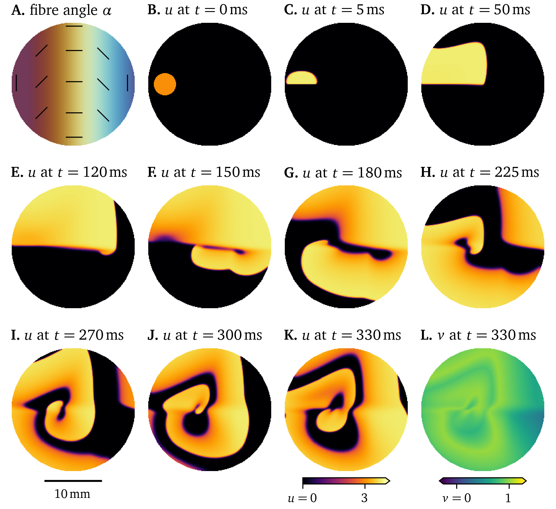
Figure 13: Simulation showing the influence of fibre direction on the wave propagation in a 6-well monolayer of the Karma model.
One way to numerically model fibrosis, i.e., regions of cells that can not be excited (Kazbanov et al., 2016), is to treat vertices in the finite-differences grid as exterior points. This was randomly done to of the vertices in the Pigreads simulation shown in Fig. 14. Here, the wave is slightly disturbed but still shows roughly the same behaviour as in the unmodified simulation (Fig. 12).
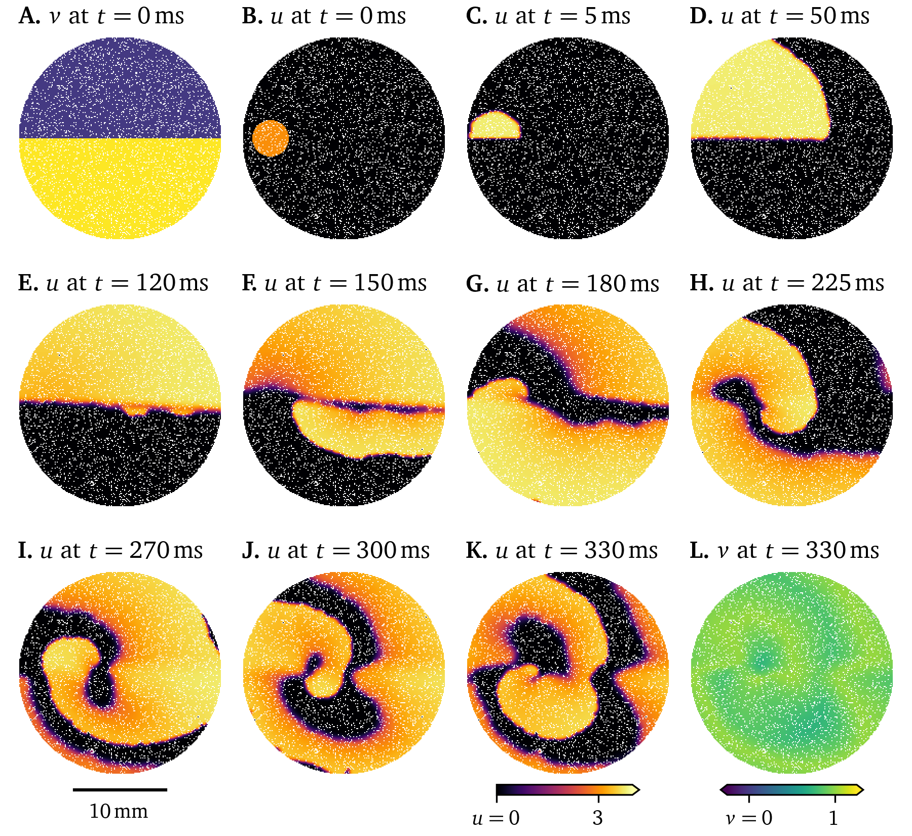
Figure 14: Simulation showing the effect of fibrosis on the wave propagation in a 6-well monolayer of the Karma model.
The deterministic dynamics of Eq. 22 are chaotic though, so small differences grow over time; the solutions diverge (A. Mitchell & Bruch Jr, 1985). Consider another simulation where a different subset of of vertices are modelled as fibrosis. While at first, the two solutions in Fig. 14 and Fig. 15 evolve in quite similar ways, the final frames show very different states.
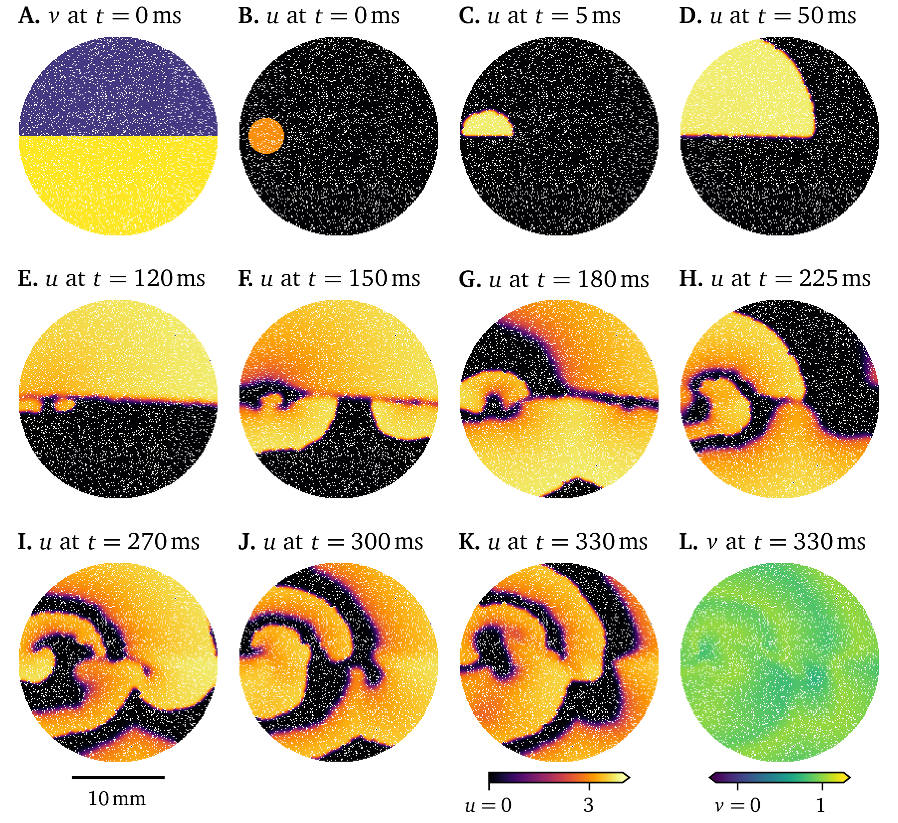
Figure 15: Simulation showing chaotic behaviour in the wave propagation in a 6-well monolayer of the Karma model. Initially small differences grow until divergence from Fig. 14.
Different types of cells, the variation between cells of the same type over space, or diseased cells may be described by changing model parameters. In the Pigreads simulation in Fig. 16, we consider an inhomogeneity at the centre of the domain, where the model parameter $\epsilon$ of the Karma model as formulated in Marcotte & Grigoriev (2017) is increased by . This leads to a quicker recovery in that region, such that the rotor is sped up. This, in turn, drives the formation of more rotors across the domain. The break up of this single spiral into multiple rotors can be interpreted as a model of tachycardia evolving into fibrillation (section 1).
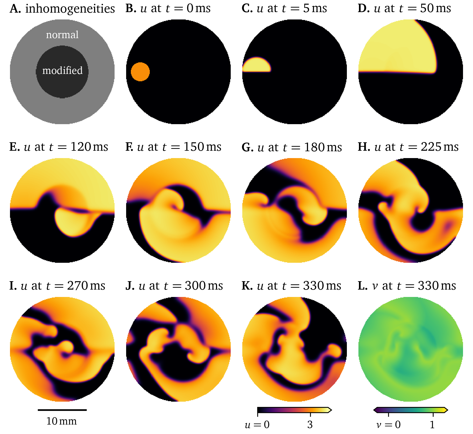
Figure 16: Simulation with inhomogeneous restitution parameters influencing the wave propagation in a 6-well monolayer of the Karma model.
Another useful inhomogeneity is to use different, but compatible cell models for different types of cells. For instance, the model by ten Tusscher & Panfilov (2006) shows slightly different behaviour for cells in the ventricular epicardium—the outside surface of the ventricles, endocardium—the inside surface, and in the middle of the ventricular wall. A sketch-like simulation that emphasises these slight differences in the excitation along with pronounced stronger diffusion along fibres in the horizontal axis can be found in Fig. 17. Due to the differences between the epi- and endocardial variants of the model, the symmetry of the wave front is broken. Models that differ may also have numerically unstable behaviour at the interfaces between them. As these models differ only slightly, they are still compatible.
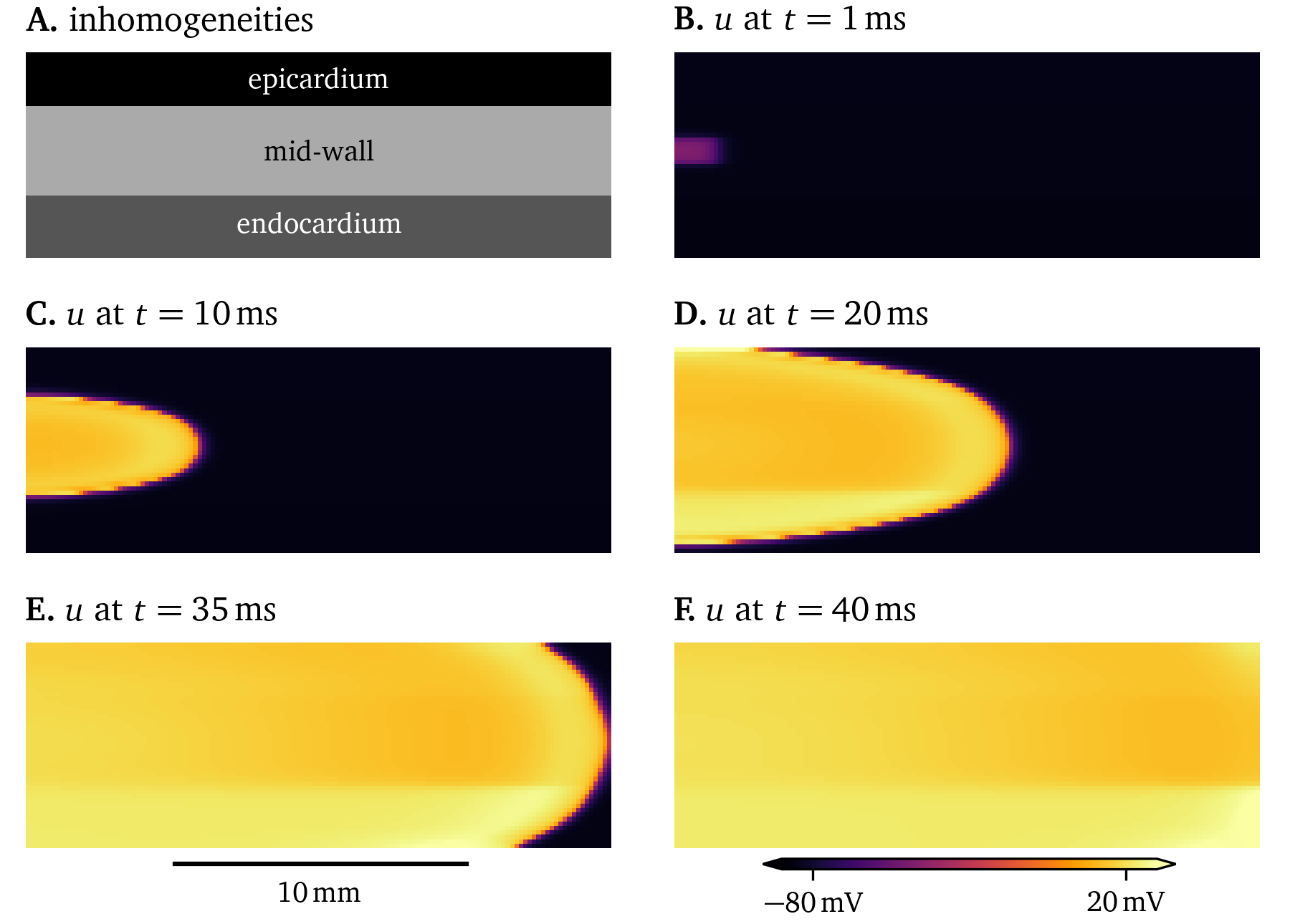
Figure 17: Simulation of a 2D domain representing a cross-section of the ventricular wall with different variants of the model by ten Tusscher & Panfilov (2006). It can be seen that the excitation is different between variants.
Detailed, ionic models of cardiac electrophysiology
Where the phenomenological models (section 2.4.3) strive for simplicity and faithfulness at the tissue level, this often comes at the cost of accuracy at the single cell level. This is in contrast to the design goals of ionic models (Courtemanche et al., 1998; Majumder et al., 2016; Paci et al., 2013; ten Tusscher & Panfilov, 2006), where it ideally includes all ionic currents and other mechanisms that effect the electrophysiological behaviour of cardiac myocytes and other excitable cells.
To create such a model, most authors adapt an existing model by optionally modifying the model equations, such that more mechanisms in the cells at hand are captured, followed by tweaking the model parameters with data from a variety of sources: Patch-clamping is usually used to record current-voltage curves that capture how a current across the cell membrane is affected by the transmembrane voltage $u$. Also obtained from patch-clamping, activation/inactivation curves can provide insight into when and how quickly the ion channel gates open in a model. Action potential duration and conduction velocity restitution curves are also used to fit such an ionic model, which may be obtained from optical mapping. Details on these methods can be found in section 1.3.
The main ion current $I_\text{ion}(t, {{\bm{{x}}}})$ in the domain ${{\bm{{x}}}}\in\heartsuit$ over time $t\in[0,T]$ typically consists of a sum of individual currents similar to the following (Courtemanche et al., 1998; Hodgkin & Huxley, 1952): $$ I_\text{ion} = I_\text{Na} + I_\text{K} + I_\text{Ca} + ... \qquad{(31)}$$ plugging into the bi- or monodomain equations (Eq. 12 or Eq. 20). The currents $I_\star(t, {{\bm{{x}}}})$ are often defined as the product of scalar conductances $G_\star$, unit-less gating variables $g_{\star, a}(t, {{\bm{{x}}}})$, and the displacement of the transmembrane voltage $u$ from the equilibrium potentials $u_{\star}(t, {{\bm{{x}}}})$ (Courtemanche et al., 1998; Hodgkin & Huxley, 1952): $$ I_\star = G_\star {{\left[ u - u_{\star} \right]}} \prod_a g_{\star a} \qquad{(32)}$$
The equilibrium potential $u_{\star}(t, {{\bm{{x}}}})$ for an ion species, e.g. Na+ , K+ , Ca2+ , etc., can be calculated as (Courtemanche et al., 1998): $$ u_{\star} = \frac{R T}{Z F} \log\frac{{{\left[ \star \right]}}_\text{e}}{{{\left[ \star \right]}}_\text{i}} \qquad{(33)}$$ with the extra- and intracellular ion concentrations ${{\left[ \star \right]}}_\text{e, i}(t, {{\bm{{x}}}})$, the valence $Z$ of the ion, temperature $T$ in ${\mathrm{K}}$, the gas constant $R = {8.3143~\mathrm{{J}{/}{K}{/}{mol}}}$, and Faraday constant $F = {96486.7~\mathrm{{C}{/}{mol}}}$.
Ion gates $g_{\star a}(t, {{\bm{{x}}}})$ can be modelled as (Courtemanche et al., 1998): $$ \partial_t g_{\star a} = \frac{ g_{\star a \infty} - g_{\star a} }{ \tau_{\star a} } \qquad{(34)}$$ with the steady state $g_{\star a \infty}$ and time scale $\tau_{\star a}$.
For gating variables following Eq. 34, instead of using an forward Euler scheme Eq. 24, one can use the Rush-Larssen time stepping scheme (Courtemanche et al., 1998; Rush & Larsen, 1978): $$ g_{\star a} \leftarrow g_{\star a \infty} + [ g_{\star a} - g_{\star a \infty} ] {{\mathrm{e}^{-\frac{\Delta t}{\tau_{\star a}}}}} \qquad{(35)}$$
It is common in the ionic models to, besides the transmembrane voltage $u$, have gating variables $g_{\star, a}$ and ion concentrations ${{\left[ \star \right]}}_\text{e, i}$ as state variables ${{\underline{{u}}}}(t, {{\bm{{x}}}})$. To keep the number of state variables as low as possible, the other quantities in Eqs. 31-34 are expressed in terms of ${{\underline{{u}}}}$.
Ionic models aim to capture the behaviour of a specific type of cell or cell line. For example, the 21-variable model by Courtemanche et al. (1998) is designed for human atrial myocytes, while the 18-variable atrial model by Paci et al. (2013) describes human induced pluripotent stem cell derived cardiomyocytes (hiPSC-CMs) in an atrial-like phenotype. Tissue-level simulations for both of these are presented in Figs. 18, 19. To stimulate a rotor in these two simulations, an S1S2 protocol was used: When the wave back of an initial stimulus (S1) is sensed at a sensor location, a second stimulus is placed, such that the new excitation wave closely follows the wave back, creating a rotor. A visualisation of this protocol can also be found in Fig. 2.5. We here use current-based stimuli, essentially an additional source term on the right-hand-side of Eq. 22 A. For the simulation of the model by Paci et al. (2013) in Fig. 19, we use an additional stimulus (S0) before the protocol as, due to the restitution properties, the action potential duration of the first pulse is much longer than that of the second pulse. In the resulting wave dynamics of the two models, it can be seen how different two models for different cell lines behave even when both of them are designed as models for the same organ, in this case the atria.
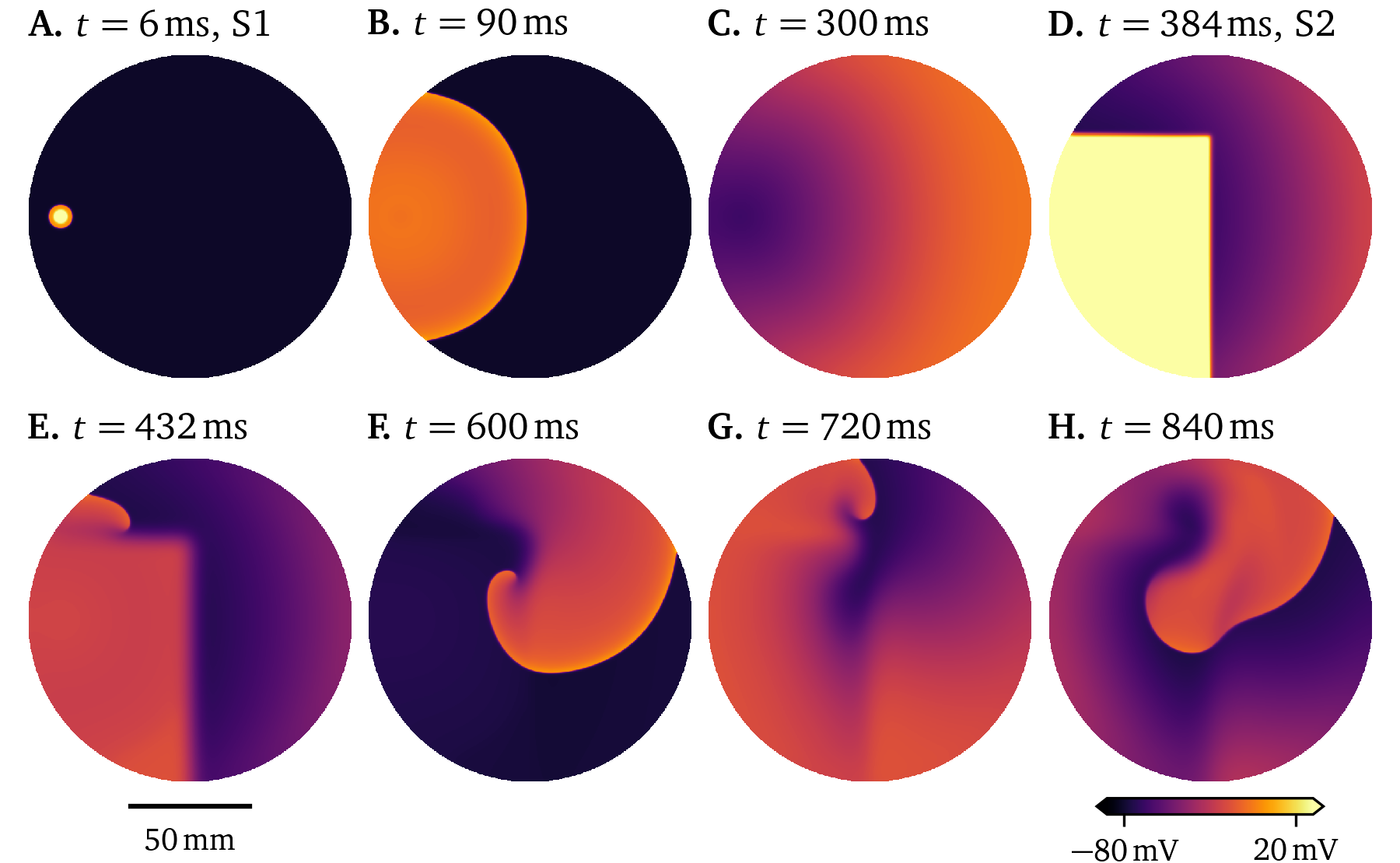
Figure 18: Simulation of the model by Courtemanche et al. (1998) in a large culture dish stimulated twice following an S1S2 protocol. A meandering rotor is formed by the second stimulus at the wave back.
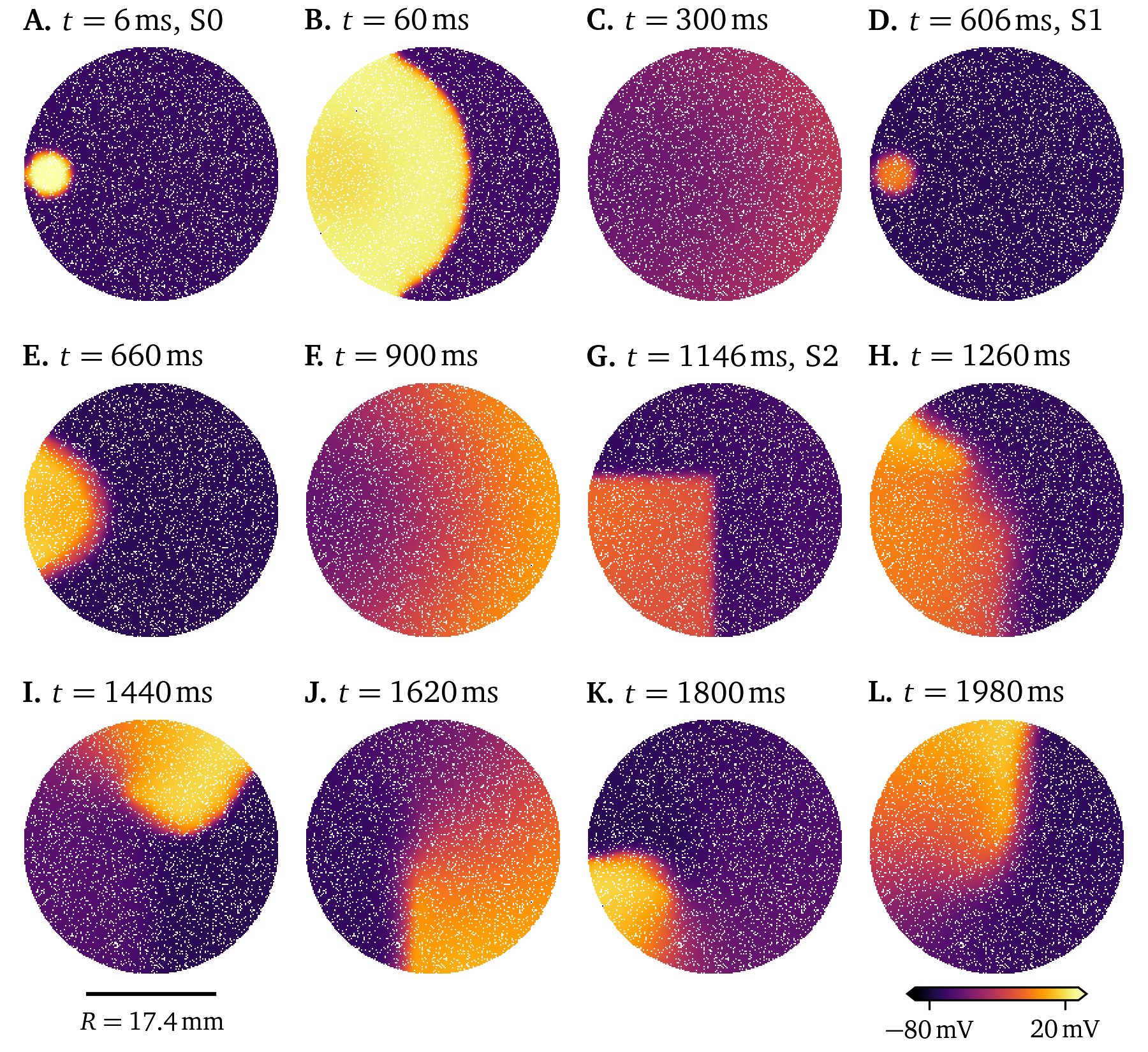
Figure 19: Simulation of the atrial model by Paci et al. (2013) in a 6-well culture dish stimulated three times following an S0S1S2 protocol. The well is just big enough to fit one rotor.
Limitations and alternatives
The in-silico models in the monodomain description presented in this section are powerful tools for studying the complex wave dynamics in heart muscle tissue. While here, we have shown simulations mostly on homogeneous and isotropic 2D discs to model monolayers, higher-dimensional simulations with anisotropy and heterogeneities can be performed. By choosing appropriate weights for the spatial derivatives, it is also possible to support curved surfaces like for instance the thin atrial wall (Davydov et al., 2000; Dierckx et al., 2013; Kabus, Cloet, et al., 2024).
Newer ionic models capture a lot of detail on the microscopic scale, while producing realistic electrical activation patterns on the tissue scale. Using them on the whole-organ scale, would make them a useful tool in the clinical context for personalised medicine: Procedures could be tested on a cardiac digital twin of the patient before they are actually implemented to test their efficacy and their impact on the patient. However, as the available computational power is usually still not big enough to tackle such large-scale whole-heart simulations, they are currently not feasible for patient care. This is mainly due to the resolution needed in space and time, i.e., $\Delta x$ and $\Delta t$, to accurately resolve the wave front, cf. Eq. 26. Also, the number of variables in detailed models—and hence the number of model equations, negatively impacts computational costs. With a higher number of model parameters, models also require more quite diverse and extensive measurements. Measuring every current in a cell line via patch-clamping is typically not feasible to create a full ionic model, so data from previously published models are imported that are assumed to also fit well to the cell line at hand. The variation between individual cells of a cell line is also often not taken into account. Finally, the currents are often re-balanced by scaling their conductances $G_\star$ so the action potential shape, and restitution characteristics match with observations. However, as these conventional ionic models are designed on the single-cell scale, they model single cells quite well.
One of the goals of this project was to explore alternatives or modifications to these conventional in-silico models of cardiac electrophysiology. High-resolution optical voltage mapping recordings of electrical activation patterns on the tissue scale (section 1.3.2) hold promise to enable fully-automatic, data-driven generation of electrophysiological models directly on the tissue-level. In the research paper presented in chapter 5, we explore one such method that can be used to quickly generate data-driven tissue excitation models from optical mapping data using a simple low-order polynomial model.
This method and other alternative models use machine learning techniques some of which will be presented in section 4. In section 3, we introduce methods that are useful to study the excitation patterns that can be observed in-vitro—in optical mapping data, as well as in-silico—the models that have been introduced in this section. These tools are used in the method presented in chapter 5.
Phase analysis of electrical activation patterns
Consider a model ${{\underline{{r}}}}({{\underline{{u}}}})$ in the single cell context, i.e., Eq. 22 with no spatial coupling ${{\bm{{D}}}} = 0$. Most of the models we consider in the context of cardiac electrophysiology capture both depolarisation and repolarisation—i.e., excitation and recovery. For a deterministic, continuous model function ${{\underline{{r}}}}({{\underline{{u}}}})$ to describe this behaviour, it is typically encoded in at least two variables ${{\underline{{u}}}} = {{{{\left[ u, v \right]}}}^\mathrm{T}}$. The variables of a model span the so-called state space. In state space, the model function is a vector field that describes the reaction at each possible state of the cells.
Phase analysis is a useful tool to understand the behaviour of a model by describing its state with a simple clock-like periodic variable—a so-called phase or phase angle ${\varphi}$. This section will introduce the main concepts of phase, phase singularities, phase defects, and their relation to conduction blocks. Phase defects are the main topic of two more scientific articles included in this dissertation, Kabus et al. (2022) in chapter 3 and Arno et al. (2024a) in chapter 4.
State space and phase
As an example, consider the reaction term ${{\underline{{r}}}}({{\underline{{u}}}}) = {{{{\left[ r_u, r_v \right]}}}^\mathrm{T}}$ of the simple two-variable model by Aliev & Panfilov (1996): $$ \begin{aligned} r_u &= - k u {{\left[ u - a \right]}} {{\left[ u - 1 \right]}} - u v & \;\;\;\text{(A)} \\ r_v &= - \epsilon v - \epsilon k u {{\left[ u - a - 1 \right]}} & \;\;\;\text{(B)} \\ \epsilon &= \epsilon_0 + \frac{\mu_1 v}{u + \mu_2} & \;\;\;\text{(C)} \end{aligned} \qquad{(36)}$$ with constant scalar parameters $k$, $a$, $\epsilon_0$, $\mu_1$, and $\mu_2$.
At each point ${{\underline{{u}}}} = {{{{\left[ u, v \right]}}}^\mathrm{T}}$ of the state space, this defines a unique reaction of the cells. This reaction is visualised as a vector function plot in Fig. 5.2. This figure is also coloured by the component of the reaction term in $u$-direction, $r_u$, or in the slightly different notation of that article $R_u$. For a starting state of $u=0.15$ and $v=0$, following the reaction ${{\underline{{r}}}}$ yields the trajectory ${{\underline{{u}}}}(t)$ drawn in black—the path following ${{\underline{{r}}}}$ through state space. It describes an arc around the state space, returning to the stable resting point, an attractor at $u=0$ and $v=0$. Small perturbations from this point lead to a restoring force towards the point. Diffusion and stimulus currents can be seen as additional source terms for $u$, see also Eq. 22. These offsets can raise $u$ above the critical threshold $a$ such that the system follows a similar trajectory to the aforementioned drawn one.
Therefore, under excitation, for instance from stimuli or in a spiral wave as in Fig. 12 or Fig. 2.5, the system’s state ${{\underline{{u}}}}$ evolves along a loop-like trajectory. This so-called inertial manifold (Temam, 1990) or dynamical attractor is visualised in Fig. 5.3 by colouring each point in the state space by how often it was visited in a two-dimensional monodomain simulation of the model by Aliev & Panfilov (1996). States near the dynamical extractor evolve towards and follow it (Cross & Hohenberg, 1993; Keener, 2004; Mikhailov et al., 1994). Encircled by the loop-like inertial manifold is a region—a “hole”—which contains significantly less likely states, i.e., ${{\underline{{u}}}}$ that the system in a normal excitation pattern does not evolve towards. We call this region of unlikely states the forbidden region in the state space (Arno et al., 2021).
Under repeated excitation, the system keeps evolving around in this loop in state space. So, with these cyclic trajectories in state space, it is natural to describe the system using an angle. This so-called phase describes the position on the cycle in state space. For a given state space evolution ${{\underline{{u}}}}(t, {{\bm{{x}}}})$ over time $t \in [0, T]$ for each point ${{\bm{{x}}}} \in \heartsuit$ in the medium, we get a function ${\varphi}(t, {{\bm{{x}}}})$. We choose ${\varphi}= 0$ as the phase at the resting state, and from there, it increases monotonously going around the loop, returning to ${\varphi}= 2\pi = 0$ (mod $2\pi$). The phase can be thought of as a “clock” for the state of the cells. A small phase value means that the system just excited, a large value closer to $2\pi$ means that the system is recovering or recovered. The details of this depend on the chosen definition of phase.
One such definition for phase is the classical phase or activation phase as an angle in state space (Bray & Wikswo, 2002; Clayton et al., 2006; R. A. Gray et al., 1998): $$ {\varphi}_\text{act} = \operatorname{arctan2}{{\left( R - R_*, V - V_* \right)}} + c \qquad{(37)}$$ where $V$ is a variable encoding the excitation of the system—typically the transmembrane voltage $u$, and $R$ is the restitution variable encoding the recovery of the system. $R_*$ and $V_*$ are constant threshold values inside the cycle’s forbidden zone, and $c$ is an offset which is typically chosen such that ${\varphi}= 0$ corresponds to the resting state.
For the definition of the restitution variable $R$, there are a few options, which all come with their advantages and disadvantages in describing the state of the system: One option is to use another state variable from ${{\underline{{u}}}}$ as the restitution variable, $R = v$. This is a common choice, particularly for two-variable models such as the models by Aliev & Panfilov (1996) or C. Mitchell (2003). If there are more than two state variables, the angle in any 2D plane in that model’s state space may be used. In Table 3.1, it can be seen that for the model by Bueno-Orovio et al. (2008), the authors choose to use the state variables $w$ and $s$ as $V$ and $R$ respectively, despite both of these variables having a less intuitive interpretation than the transmembrane voltage $u$ (Kabus et al., 2022). Another option is to extract $R$ from the temporal evolution of $V$, e.g., $R$ as a time delayed version of $V$ (R. A. Gray et al., 1995). This has the advantage to work when only a single state variable $V$ of the system can be observed. Alternatively, the Hilbert transform of $V$ may be used as $R$ (Bray & Wikswo, 2002), or the exponential moving average, see Eq. 6, (Kabus, De Coster, et al., 2024). This has the advantage to be more robust to noise.
Another way to define the phase is via the LAT, see section 1.1. The LAT at each point ${{\bm{{x}}}} \in \heartsuit$ over time $t \in [0, T]$ can be defined as the last time $t$, at which $V$ rose over a threshold $V_*$: $$ t_\text{LAT} ({{\bm{{x}}}}, t) = \operatorname{argmax}_{t' \le t} {{\left\{V ({{\bm{{x}}}}, t') = V_* \wedge \partial_t V ({{\bm{{x}}}}, t') > 0 \right\}}} \qquad{(38)}$$ LAT maps can, in the clinical context, be measured from catheter recordings in the heart (Cantwell et al., 2015), see also section 1.3.2. These maps are then used to identify conduction block lines (CBL), i.e., lines on the surface of the heart muscle that the conduction wave does not cross. CBLs are linked to arrhythmogenesis (Ciaccio et al., 2016), i.e., the formation of heart rhythm disorders, such as tachycardia and fibrillation (section 1).
An LAT-based phase can be defined as (Arno et al., 2021): $$ {\varphi}_\text{LAT} ({{\bm{{x}}}}, t) = f(t - t_\text{LAT} ({{\bm{{x}}}}, t)) \qquad{(39)}$$ with a scaling function $f: [0,\infty) \rightarrow [0,2\pi]$, such that: $$ \begin{aligned} f(0) &= 0 \\ \lim_{\tau \to \infty} f(\tau) &= 2 \pi \\ \forall \tau: f'(\tau) &\ge 0 \end{aligned} \qquad{(40)}$$ These properties ensure that the LAT-based phase has the properties we expect from a phase to be monotonously increasing from the resting state at ${\varphi}= 0$. As the time since last excitation increases, we expect ${\varphi}$ to approach a value close to $2\pi$. For a characteristic time $\tau_0$ of recovery, choices for this scaling function $f$ are $f(\tau) = 2\pi \tanh {{\left( \frac{\tau}{\tau_0} \right)}}$ (Arno et al., 2021; Kabus et al., 2022), or $f(\tau) = \frac{2\pi\tau}{\tau_0}$, clipped to the range $[0, 2\pi]$ (Arno et al., 2024a).
In Fig. 3.3, the different phase definitions are visually compared. For the state space phase ${\varphi}_\text{act}$ (Eq. 37), points where all phases meet can be found at at the centres of spiral waves; while the LAT-based phase ${\varphi}_\text{LAT}$ (Eq. 39) exhibits discontinuous jumps, e.g. at conduction block lines. So, the different phase definitions give us different points of view on the nature of spiral wave cores.
Phase singularities and phase defects
There are two different but related ways of describing the centres of spiral waves—also referred to as rotor cores: Phase singularities (PSs) are located where all phases meet (R. A. Gray et al., 1998), while phase defects (PDs) are those points where the phase exhibits a discontinuous jump (Arno et al., 2021; Tomii et al., 2021). PSs have co-dimension 2, meaning that in two spatial dimensions, they are points, and in three dimensions, they are lines which are called filaments. PDs have co-dimension 1, so in 2D, they are phase defect lines (PDLs) and in 3D, they are ribbon-like phase defect surfaces (PDSs) (Arno et al., 2021, 2024b).
In Fig. 20, the relation between PSs and PDs is illustrated for a Pigreads simulation of the Karma model. In this example, the phase was calculated for the two phase definitions (Eqs. 37, 39), then the cosine method (Tomii et al. (2021), Kabus et al. (2022)), which will be introduced in chapter 3 (Eq. 3.12), is used to find jumps in the phase. In the state space phase ${\varphi}_\text{act}$, PSs can be seen, in contrast to the extended PDLs in ${\varphi}_\text{LAT}$.
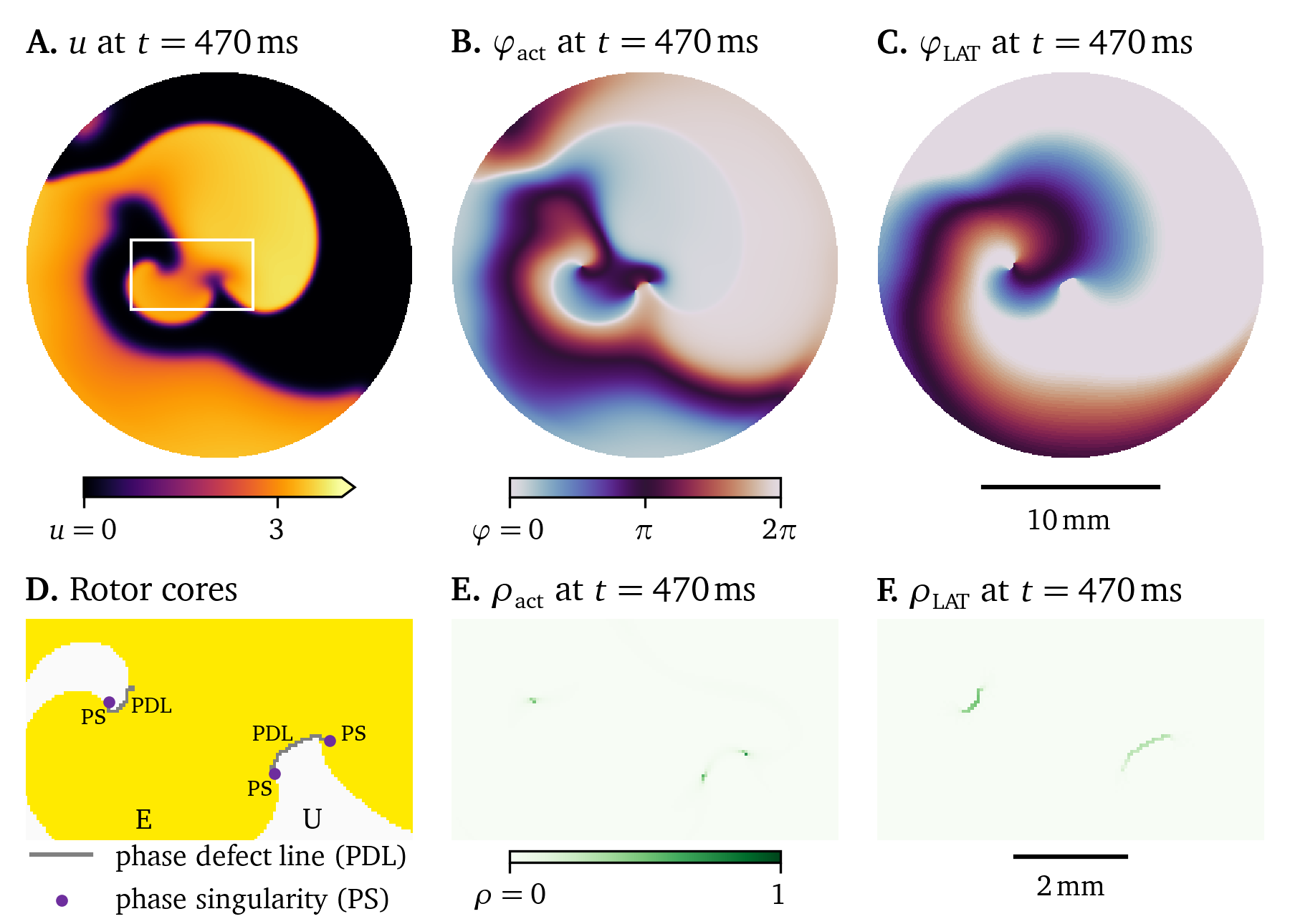
Figure 20: Phase singularities and defects in a simulation of the Karma model. Different phase definitions were used to convert the recordings in the variables $u$ (panel A.) and $v$, to the state space phase ${\varphi}_\text{act}$ (Eq. 37, panel B.), or the LAT phase ${\varphi}_\text{LAT}$ (Eq. 39, panel C.). The cosine method was used to find discontinuities in the phases (Eq. 3.12, panels E and F, respectively). For the state space phase, point-like PSs can be seen, while for the LAT phase, extended PDLs can be seen (panel D.). Note that the two PSs on the right lie on the same PDL, a conduction block line. The region considered excited is coloured yellow and labelled “E” in panel D, the unexcited region is labelled “U”.
In Fig. 2.10, a similar view is provided in 3D for the model by Bueno-Orovio et al. (2008). The PDSs are ribbon-like surfaces, here identified with a method that ascribes them with finite thickness and filament lines.
Re-entrant waves can form around an inhomogeneity in the medium—like an obstacle—which is called anatomical re-entry, but they can also exist in homogeneous tissue, where the rotor is not anchored to an obstacle in so-called functional re-entry (Fenton et al., 2000). The overall behaviour of a rotor is mainly driven by its core; if the core is undisturbed, the rotor will persist. Describing re-entry as PSs or PDs can offer deeper insights into the interactions of rotors with one another, how re-entrant circuits multiply and how they can be removed. For instance, re-entry that keeps forming around the same obstacle can be prevented via ablation: Locate the in-excitable obstacle, for instance as PDLs in LAT mapping recordings, and make more tissue in-excitable, for instance by burning or freeze-burning, such that afterwards, no more anatomical re-entry is possible around the new obstacle (Deisenhofer et al., 2010; Haissaguerre et al., 1998).
The detection of PDs is the topic of chapter 3, which was also published as a scientific research paper (Kabus et al., 2022). In chapter 4, another research paper published as part of this dissertation (Arno et al., 2024a), the interactions of PDLs, wave fronts and backs are for the first time studied as quasiparticles with Feynman diagrams, a sketch of particle interactions from the field of particle physics. The arising quasiparticles are further studied in up-coming research by Gobeyn et al. (in preparation).
Machine learning techniques for creating data-driven excitation models
The long-term goal of computational medicine is to create personalised digital twins—a high-detail, high-fidelity, high-resolution representation of entire organs or even the entire body of a patient (Niederer et al., 2019; Trayanova et al., 2020). A digital twin would allow testing treatments on it first to evaluate their effectiveness and impact before actually performing them on the patient. An ideal, full digital twin for cardiac electrophysiology would enable faster-than-real-time simulations of the electrical activation patterns based on all available measurements of a patient’s heart, such as its geometry, or electrocardiograph (ECG), EGM, and mapping recordings. An ideal digital twin would be fully data-driven, i.e., a model of the heart is created from minimal assumptions extracting all relevant information about the dynamics from the data.
There are two fundamental challenges in creating such data-driven digital twins:
- Making use of as much of the available data as possible.
- Designing numerical methods that are sufficiently fast for clinical applications.
Regarding the first point of inclusion of more data, note that most in-silico models of cardiac electrophysiology are fitted using fairly little data—mainly patch clamping and restitution curves, as we have discussed in section 2.7. The model fitting procedure also typically requires human input and is far from automated. This makes these conventional models a suboptimal starting point in the design of digital twins: They are both not data-driven and can not easily be created automatically.
Regarding the second point of computational cost, in section 2.3, we have seen that the numerical solution of a reaction-diffusion system—a system of partial differential equations (PDEs)—requires adequate resolution in space and time for numerical stability (Courant et al., 1928). In the context of cardiac electrophysiology, the computational effort to resolve those systems of equations is therefore quite high making them too slow for clinical applications with the currently available computers: For larger tissue volumes, resolutions are required to be roughly in the order of $\Delta x \approx {0.1~\mathrm{{m}{m}}}$ in three spatial dimensions and $\Delta t \approx {0.01~\mathrm{{m}{s}}}$ in time (Clayton et al., 2011). As an order-of-magnitude estimate, at this resolution, a reaction-diffusion simulation of of an organ in size would require calculations of the reaction term and the Laplacian on 1014 nodes in space and time, i.e., 100 trillion nodes. A possible workaround to reduce the computational cost is to use a surrogate model, i.e., an algorithm producing good approximations of the original model while, ideally, being much more computationally efficient (Raissi et al., 2019).
With the tools from machine learning, many options for the design of surrogate models and digital twins are opened up. In this section, we present some of these possible options after we introduce some of the basic methods which they build upon.
The learning problem
As a general optimisation problem consider an unknown function ${{\bm{{y}}}} = \hat f({{\bm{{x}}}})$—the target function—and a data set of $N$ pairs of input and output vectors: the inputs ${{\bm{{x}}}}_n \in \mathcal X$, indexed by $n \in {{\left\{1, ..., N \right\}}}$ and corresponding outputs ${{\bm{{y}}}}_n \in \mathcal Y$ (Abu-Mostafa et al., 2012). We now are looking for the optimal function $f \in \mathcal F$ which fits these data ${{\bm{{y}}}}_n \approx f({{\bm{{x}}}}_n)$ within a set of possible candidate functions $\mathcal F$, the hypothesis set. This process is called fitting the function $f$, optimising the function, or even “learning” the function. Except for the simplest cases, this is usually done with computers, hence the field of function optimisation is often called machine learning.3
More specifically, the problem of finding a function $f$ given annotated data, points ${{\bm{{x}}}}_n$ and labels ${{\bm{{y}}}}_n$, such that ${{\bm{{y}}}}_n \approx f({{\bm{{x}}}}_n)$, is called supervised machine learning. This is in contrast to unsupervised machine learning, in which patterns in unlabelled data ${{\bm{{x}}}}_n$ should be discovered. Unsupervised machine learning tasks are for instance finding clusters in data, measuring the similarity of data, or finding trends in the data. Supervised and unsupervised machine learning are often used together, for instance, one can use principal component analysis to transform high-dimensional data onto a space with fewer dimensions in which the data have the most variance. In this lower-dimensional space, the set of function candidates to be searched for an optimal solution is then also smaller.
A common way to state the so-called learning problem of supervised machine learning is in terms of a loss function $\mathcal L$ which is defined such that it is minimal for the optimal choice of $f \in \mathcal F$, for instance: $$ \mathcal L(f) = \frac {1}{N} \sum_{n=1}^N l{{\left( {{\bm{{y}}}}_n, f({{\bm{{x}}}}_n) \right)}} \qquad{(41)}$$ using a distance function $l : \mathcal Y \times \mathcal Y \to \mathbb R$ in the output space $\mathcal Y$, e.g.: $$ l({{\bm{{y}}}}_a, {{\bm{{y}}}}_b) = {{\left\lVert {{\bm{{y}}}}_a - {{\bm{{y}}}}_b \right\rVert}} \qquad{(42)}$$
Many optimisation problems in supervised machine learning then take the following form:
Given $N$ data ${{\bm{{x}}}}_n \in \mathcal X$ and ${{\bm{{y}}}}_n \in \mathcal Y$, find the function $f\in\mathcal F$ in the hypothesis set which minimises the loss function $\mathcal L$ (Eq. 41).
While the learning problem can be stated in more general forms, this version suffices for the methods introduced in the following.
Least-squares method
As a more concrete example of an optimisation problem, consider $N$ data points ${{\bm{{x}}}}_n \in \mathcal X \subseteq \mathbb C^{D + 1}$ in $D$ dimensions, indexed by $n \in {{\left\{1, ..., N \right\}}}$ and $d \in {{\left\{0, 1, ..., D \right\}}}$, and corresponding observed scalar function values $y_n \in \mathcal Y \subseteq \mathbb C$, sampled from an unknown target function $y_n = \hat f({{\bm{{x}}}}_n)$. For simpler notation, we define the zero-th element of all vectors ${{\bm{{x}}}}_n$ to be equal to one, i.e., $\forall n: x_{n, 0} = 1$.
One of the simplest classes of functions in this form are linear functions, i.e., the linear regression model, using a vector of weights ${{\bm{{w}}}} \in \mathcal W \subseteq \mathbb C^{D+1}$: $$ y_n \approx f({{\bm{{x}}}}_n) = {{{{\bm{{w}}}}}^\mathrm{T}}{{\bm{{x}}}}_n \qquad{(43)}$$ Due to the convention of defining $x_{n,0} = 1$, the zero-th element in the weight vector $w_0$ takes the function of a so-called bias; the entire function $f$ is shifted by this offset. For this hypothesis set, each point in the parameter space ${{\bm{{w}}}} \in \mathcal W$ maps to a function $f \in \mathcal F$.
For the hypothesis in Eq. 43 and Euclidean distance in $\mathcal Y$, the loss function Eq. 41 then takes this form (Abu-Mostafa et al., 2012): $$ \mathcal L({{\bm{{w}}}}) = \frac {1}{N} \sum_{n=1}^N {{\left\lVert y_n - {{{{\bm{{x}}}}}^\mathrm{T}}_n{{\bm{{w}}}} \right\rVert}}^2 = \frac {1}{N} {{\left\lVert {{\bm{{y}}}} - {{\bm{{X}}}} {{\bm{{w}}}} \right\rVert}}^2 \qquad{(44)}$$ where we have re-written the right-hand side using the matrix of all data points ${{\bm{{X}}}} \in \mathbb C^{N\times(D+1)}$, again with the convention that $\forall n: x_{n,0} = 1$.
To find the optimal choice of the weights ${{\bm{{w}}}}$, the parameters of the hypotheses functions, we minimise the loss by finding the weights for which the gradient of the loss is zero (Abu-Mostafa et al., 2012): $$ \begin{aligned} {{\bm{{0}}}} &= N \nabla_{{{\bm{{w}}}}} \mathcal L({{\bm{{w}}}}) = \nabla_{{{\bm{{w}}}}} {{\left\lVert {{\bm{{y}}}} - {{\bm{{X}}}} {{\bm{{w}}}} \right\rVert}}^2 = {{{{\bm{{X}}}}}^\mathrm{T}} {{\left( {{\bm{{y}}}} - {{\bm{{X}}}} {{\bm{{w}}}} \right)}} \\ \Rightarrow {{\bm{{w}}}} &= {{\left[ {{{{\bm{{X}}}}}^\mathrm{T}} {{\bm{{X}}}} \right]}}^{-1} {{{{\bm{{X}}}}}^\mathrm{T}} {{\bm{{y}}}} \end{aligned} \qquad{(45)}$$
Therefore, to fit a linear regression with the least-squares method (Eq. 45), only matrix multiplication and matrix inversion operations are needed; this is usually realised using Gaussian elimination. The least-squares method gets its name from the minimisation of a loss function that is the sum of squared distances, as sketched in Fig. 21. Least-squares is a very robust method due to the straight-forward use of common matrix operations and its lack of super-parameters. It is used as a component of many other optimisation methods when a linear function needs to be fitted.
Figure 21: Sketch of linear and parabolic least-squares fits. This optimisation method finds the linear function (solid line) that minimises the sum of the squares of the distances between predicted and true output values $y$. The data have been sampled from the target function (dotted) with random Gaussian additive noise. Despite being sampled from a linear function, the fitted parabola (dashed) has a lower loss function value.
Polynomial fitting
The least-squares method can, for instance, be used to not just fit linear functions to data ${{\bm{{x}}}} \in \mathcal X \subseteq \mathbb C^{D + 1}$ and $y \in \mathcal Y \subseteq \mathbb C$, but any polynomial of finite degree, such as: $$ \begin{aligned} f({{\bm{{x}}}}) = f(x_1, x_2) = w + w_1 x_1 + w_2 x_2 + w_{11} x_1^2 + w_{12} x_1 x_2 + w_{22} x_2^2 \\ f({{\bm{{z}}}}) = w z_0 + w_1 z_1 + w_2 z_2 + w_{11} z_{11} + w_{12} z_{12} + w_{22} z_{22} \end{aligned} \qquad{(46)}$$ Note that this polynomial is just a linear function with respect to the polynomial expansion ${{\bm{{z}}}}({{\bm{{x}}}})$ of the data, which, in this case, is defined as: $$ {{\bm{{z}}}}({{\bm{{x}}}}) = {{{{\left[ z_0, z_1, z_2, z_{11}, z_{12}, z_{22} \right]}}}^\mathrm{T}} = {{{{\left[ 1, x_1, x_2, x_1^2, x_1 x_2, x_2^2 \right]}}}^\mathrm{T}} \qquad{(47)}$$
Fitting a polynomial of a given degree can therefore be done by applying the corresponding polynomial transform to the input data ${{\bm{{x}}}}$ followed by applying the least-squares method to find a linear function to the transformed data ${{\bm{{z}}}}$, $y$. In Fig. 21, a parabola is also fitted to the data using polynomial expansion and the least-squares method.
Neural networks
The central idea behind neural networks is to approximate complex functions by combining many simple functions. This is captured in the universal approximation theorem, which states that a sufficiently complex neural network can approximate any continuous function given enough data (Hornik et al., 1989). Neural networks are inspired by the brain: Neurons are arranged in a network and, when stimulation by its neighbouring input neurons is strong enough, a neuron can fire which may, in turn, stimulate other neurons.
As sketched in Fig. 22, a neural network ${{\bm{{y}}}} = f({{\bm{{x}}}})$ consists of $L$ layers of neurons, i.e., nodes, indexed by $\ell \in \{0, ..., L\}$ and $d \in \{0, ..., D_\ell\}$. The value of the zeroth layer is set to the input, ${{\bm{{x}}}}_{0} = {{\bm{{x}}}} \in \mathbb C^{D_x+1}$; while the output of the $L$th layer is the output of the neural network, ${{\bm{{y}}}} = {{\bm{{x}}}}_L \in \mathbb C^{D_y+1}$. The value $x_{\ell, d} \in \mathbb C$ of each neuron in all layers except the zeroth is calculated based on the values ${{\bm{{x}}}}_{\ell - 1} \in \mathbb C^{D_{\ell-1}+1}$ of the previous layer using a linear term with weights ${{\bm{{w}}}}_{\ell, d} \in \mathbb C^{D_{\ell-1}+1}$ and a so-called activation function $\vartheta_{\ell, d} : \mathbb C \to \mathbb C$ (Abu-Mostafa et al., 2012): $$ x_{\ell, d} = \vartheta_{\ell, d}{{\left( {{{{\bm{{w}}}}}^\mathrm{T}}_{\ell, d}{{\bm{{x}}}}_{\ell-1} \right)}} \qquad{(48)}$$ Note that again $\forall \ell: x_{\ell, 0} = 1$, such that $w_{\ell, d, 0}$ is the bias in the linear term.
Figure 22: Sketch of a fully connected feed-forward neural network. Each layer contains nodes, also known as neurons, whose value is computed based on the values of the nodes in the previous layer. Each layer contains a constant node with $x_{\ell,0} = 1$.
The activation function $\vartheta_{\ell, d}$ plays a crucial role in neural networks as a scaling function which is applied to the linear combination of inputs from the previous layer, introducing non-linearities that facilitate learning complex patterns. The choice of activation function significantly impacts a neural network’s performance, influencing both its expressiveness and the ease of training. Two widely used activation functions are the sigmoid function $\vartheta_{\text{sig}}$ and the rectified linear unit (ReLU) $\vartheta_{\text{ReLU}}$.
The sigmoid function introduces smooth, differentiable non-linearity and is defined as: $$ \vartheta_{\text{sig}}(x) = \frac{1}{1 + {{\mathrm{e}^{-x}}}} \qquad{(49)}$$ However, it can suffer from the vanishing gradient problem, which makes training deep networks challenging (Hochreiter, 1991; Hochreiter et al., 2001).
The rectified linear unit (ReLU), on the other hand, is defined as: $$ \vartheta_{\text{ReLU}}(x) = \max(0, x) \qquad{(50)}$$ While not differentiable at $x=0$, ReLU is more computationally efficient than the sigmoid function.
The weights $w_{\ell d b}$ are usually stored in a large vector ${{\bm{{W}}}}$, which is trained using an optimisation algorithm, such as stochastic gradient descent (SGD) or one of its variants. The optimisation algorithm changes the weights in the direction that minimises a loss function (Eqs. 41, 44) that quantifies the discrepancy between the output of the neural network and the target output.
To find the gradient of the loss function with respect to the weights, the back-propagation algorithm is used. It gets its name from the fact that, in contrast to forward propagation, which computes the output of the network given the input, it computes the gradient of the loss function by propagating the error backwards through the network to find how much each node has contributed to it.
At each node or neuron, the back-propagation algorithm follows the chain rule to compute the gradient of the loss with respect to the weights. To sketch out the back-propagation algorithm, recall this general form of the loss function and main equation for the output of a node (Eq. 48), rewritten using the linear terms $s_{\ell d}$: $$ \begin{aligned} \mathcal L({{\bm{{W}}}}) &= \sum_{d=0}^{D_L} c(x_{L d}, y_d) \\ x_{\ell d} &= \vartheta_{\ell d}(s_{\ell d}) \\ s_{\ell d} &= {{{{\bm{{w}}}}}^\mathrm{T}}_{\ell d} {{\bm{{x}}}}_{\ell-1} \end{aligned} \qquad{(51)}$$ For target values ${{\bm{{y}}}}$ and the predicted values ${{\bm{{x}}}}_L$, the gradient of the loss function with respect to the weights for back-propagation is given by: $$ \begin{aligned} \frac{\partial \mathcal L}{\partial w_{\ell d b}} &= \sum_{q=0}^{D_{L}} c'(x_{L q}, y_{q}) {\frac{\partial x_{L q}}{\partial w_{\ell d b}}} \\ { \frac{\partial x_{\ell d}}{\partial w_{k b q}} } &= \begin{cases} \vartheta'_{\ell d}(s_{\ell d}) \; {\frac{\partial s_{\ell d}}{\partial w_{k b q}}} & \text{if } \ell > 0 \\ 0 & \text{otherwise} \end{cases} \\ { \frac{\partial s_{\ell d}}{\partial w_{k b q}} } &= \sum_{p=0}^{D_{\ell-1}} {{\left[ w_{\ell d p} {\frac{\partial x_{\ell-1, p}}{\partial w_{k b q}}} + x_{\ell-1, p} {\frac{\partial w_{\ell d p}}{\partial w_{k b q}}} \right]}} \\ {\frac{\partial w_{\ell d b}}{\partial w_{k q p}}} &= \begin{cases} 1 & \text{if } \ell = k \text{ and } d = q \text{ and } b = p \\ 0 & \text{otherwise} \end{cases} \end{aligned} \qquad{(52)}$$ where $\ell, k$ are indices of the layers and $d, b, q, p$ are indices of the neurons in the layers. The gradient can then be calculated by first computing the values $x_{\ell d}$ and $s_{\ell d}$ for all neurons in the network using forward propagation (Eq. 51), followed by calculating the weighted sum of products in the network for each weight (Eq. 52). Only the edge with $\ell = k$ and $d = q$ and $b = p$ has a non-zero derivative with respect to the weight $w_{k q p}$, so only its and the weights of the edges “down-stream” of this node contribute to its component of the gradient.
As they are general function approximators, neural networks have a wide variety of use cases. However, it can be difficult to train them, as the number of parameters needed for many tasks can be too great to be learned from the available data, the so-called curse of dimensionality. There are several ways to address this issue, such as regularisation or using algorithms that make better use of their available parameters, such as convolutional neural networks (CNNs) for input data ${{\bm{{x}}}}$ with a grid-like structure, i.e., images or videos.
To regularise the training of neural networks, to prevent so-called overfitting, one can, for example, randomly set a percentage of the node’s values to zero during training, which is called dropout. This way, the network can not rely too heavily on any individual node. Alternatively, in so-called weight decay, one may add a term to the loss function that “penalises” large weights, e.g. the L1 or L2 norm of the vector of all weights ${{\bm{{W}}}}$.
CNNs are well-suited for images as inputs, as they can capture spatial patterns in the data using convolutional layers. These layers apply a stencil to the data that combines the values in a neighbourhood of the input data, which can extract useful features from the data. Usually, this is implemented as weighted sums of the input data. The dense layers of a CNN can then combine these local features to predict the output. CNNs have been successfully applied to a variety of computer vision tasks, such as image classification, object detection, and image segmentation. One such application is cell counting, where CNNs have been used to count the number of cells and nuclei in images of tissue samples (Van Valen et al., 2016; Weisrock et al., 2024). Due to the variability in the shapes and sizes of cells, this task is challenging using traditional image processing techniques, while CNNs can achieve performance similar to a human expert.
In summary, neural networks and their extensions are useful tools for general function approximation and have been applied to a wide range of tasks.
Physics-informed neural networks
Another promising use case of neural networks is to compute solutions $u(t, {{\bm{{x}}}})$ to PDEs of the following form, which is coined by Raissi et al. (2019) as physics-informed neural networks (PINNs): $$ \partial_t u + \mathcal D(u) = f = 0 \qquad{(53)}$$ with a nonlinear differential operator $\mathcal D(u)$ in space, to be amended with boundary and initial conditions in $u$. We define the left hand side as $f(t, {{\bm{{x}}}})$, the residual of the PDE. The solution $u(t, {{\bm{{x}}}})$ is then described using a neural network. It is the solution to this particular instance of the problem; for different initial and boundary conditions, another solution must be found and the neural network re-trained from scratch. PDEs that fulfil Eq. 53 are for instance the reaction-diffusion equation (Eq. 22) or the one-dimensional Burgers’ equation: $$ \partial_t u + u \partial_x u - c \partial_x^2 u = f = 0 \qquad{(54)}$$
As the term “physics-informed” implies, the physical knowledge of the PDE governing the system is included as regularisation terms in the to-be-minimised loss function which penalises unrealistic solutions: $$ \mathcal L = \frac {1}{N} \sum_{n=1}^N {{\left\lVert u_n - u(t_n, {{\bm{{x}}}}_n) \right\rVert}}^2 + \frac {1}{C} \sum_{c=1}^C {{\left\lVert f(t_c, x_c) \right\rVert}}^2 \qquad{(55)}$$ We here use $N$ labelled training data points $t_n, {{\bm{{x}}}}_n, u_n$; and $C$ collocation points $t_c, {{\bm{{x}}}}_c$, at which to check the PDE (Eq. 53). Additional terms can be added to enforce, for instance, boundary conditions or initial conditions.
This physics-based regularisation has the additional benefit to make this method quite robust to overfitting to the data. PINNs can also work without discretisation of domain and time. The neural network $u$ is trained as usual, for example, using gradient descent, or a quasi-Newton method, enabling the use of the robust machine learning libraries developed in the last decades. The derivatives of $u$ in the loss function can be found using automatic differentiation, i.e., the exact derivatives of the neural network can be found analytically based on the chosen network architecture. More structure can also be imposed on the neural network, for instance a forward Euler or Runge-Kutta time-stepping scheme of high order, resulting in a discrete time model (Raissi et al., 2019).
PINNs have been successfully used to solve various problems, e.g., starting with the Burgers’ equation, and Schrödinger’s equation (Raissi et al., 2019), to fluid mechanics (Cai et al., 2021), meteorology, chemical engineering, and biophysics (Toscano et al., 2024). PINNs have also been used in the context of cardiology: for the reconstruction of LAT maps from sparse recordings (Costabal et al., 2020), the reconstruction of excitation waves from mechanical deformation (Dermul & Dierckx, 2024), or as a surrogate model for reaction-diffusion systems for the model by Aliev & Panfilov (1996; Martin et al., 2022).
Another use case of PINNs is data-driven discovery of PDEs: Given data from a solution to a system of PDEs, it is possible to recover not only the solution to this system but also system parameters (Raissi et al., 2019). The data-driven discovery of PDEs via PINNs could also be applied to find cardiac electrophysiology model parameters.
Creation of data-driven cardiac excitation models
Besides the aforementioned PINN-based approaches, a variety of other machine learning techniques have been tried to create cardiac excitation models to various degrees of success. In simple terms, the goal is to approximate the dynamics described by the bi- or monodomain descriptions using more versatile and faster models that can be trained on data.
One simple approach to this task is to approximate the reaction term in the reaction-diffusion equation (Eq. 22) with a neural network: $$ \partial_t {{\underline{{u}}}} = {{\underline{{P}}}} \nabla \cdot {{\bm{{D}}}} \nabla {{\underline{{u}}}} + {{\underline{{r}}}}_\text{NN} ({{\underline{{u}}}}) \qquad{(56)}$$ However, this approach is futile because, in most cases, only some of the elements of the reaction term can be directly measured in experiments. One could however use a neural network in this way to approximate an existing model, yielding a surrogate model that, depending on the complexity of the original model, could be faster to evaluate. The numerical solution of the system remains the same though: The reaction-diffusion equation still needs to be solved and the usual constraints of the CFL condition (Eq. 26) apply. Meaning, the speed-up would only be marginal.
Another naive approach is to use a dense neural network to approximate the entire right-hand side of the reaction-diffusion equation (Eq. 22) at lower resolution in space and time: $$ \partial_t {{\underline{{u}}}} = {{\underline{{P}}}} \nabla \cdot {{\bm{{D}}}} \nabla {{\underline{{u}}}} + {{\underline{{r}}}} ({{\underline{{u}}}}) \approx \dot{{{\underline{{u}}}}}_\text{NN} {{\left( {{\left\{{{\underline{{u}}}}_n \right\}}}_{n=1}^N \right)}} \qquad{(57)}$$ where the state vectors ${{\underline{{u}}}}_n$ at $N$ points in the neighbourhood of ${{\underline{{u}}}}$ are used as input of the neural network. This approach also has some notable drawbacks: The dimension of the network’s input space is quite large as it grows with the number of points $N$ and the dimension of the state vector ${{\underline{{u}}}}$. So, the network also needs to be quite large and hence has a lot of parameters to train, requiring more data and more time for training. Also, no information about the spatial structure is used, so the network has to learn the spatial structure from scratch. There is also no information about the underlying physics, further increasing the complexity of the task.
One could remedy the latter two drawbacks by using a CNN instead of a dense network. A selection of spatial features could be extracted by convolutional layers $\hat u_\text{conv}$ and subsequently used by a dense neural network $\dot{{{\underline{{u}}}}}_\text{dense}$: $$ \partial_t {{\underline{{u}}}} = {{\underline{{P}}}} \nabla \cdot {{\bm{{D}}}} \nabla {{\underline{{u}}}} + {{\underline{{r}}}} ({{\underline{{u}}}}) \approx \dot{{{\underline{{u}}}}}_\text{dense} {{\left( \hat u_\text{conv}{{\left( {{\left\{{{\underline{{u}}}}_n \right\}}}_{n=1}^N \right)}} \right)}} \qquad{(58)}$$ This approach has the advantage that the network can be trained to learn spatial features reducing the number of parameters compared to Eq. 57. However, the network still has to learn the underlying physics from scratch. We found that the spatial features extracted can be enough to describe the diffusion term, and hence the spread of the excitation wave, but not the reaction term. The restitution characteristics of the tissue involve temporal features that are not included in the spatial features extracted by the convolutional layers. We therefore would also need to include points from previous time steps in the input of the network, increasing the dimensional complexity of the task yet again. The dense network would get both spatial and temporal features as input.
Now, we propose to only use features that are known to be relevant for excitation waves in cardiac electrophysiology. For the purposes of this project, this is the approach that gave the best results. In a first prototype with code name Melange, we used a dense neural network to approximate the reaction-diffusion equation (Eq. 22) with a reduced set of features extracted from optical voltage mapping data:
- the transmembrane voltage $u$, proportional to the change in observed light intensity,
- approximate monopolar EGMs $u_\text{EGM}$ (Eq. 9),
- a moving average $\tilde u$ of the transmembrane potential $u$ over the last few time steps (Eq. 6),
- the absolute value ${{\left\lVert \nabla u \right\rVert}}$ of the gradient of the transmembrane voltage,
- the local activation time phase ${\varphi}_\text{LAT}$ (Eq. 39),
- the APD of the most recent pulse (Eq. 1),
- and DI between the two most recent activations (Eq. 2).
Or, expressed as a PDE: $$ \partial_t {{\underline{{u}}}} = {{\underline{{P}}}} \nabla \cdot {{\bm{{D}}}} \nabla {{\underline{{u}}}} + {{\underline{{r}}}} ({{\underline{{u}}}}) \approx \dot{{{\underline{{u}}}}}_\text{Melange} {{\left( u, u_\text{EGM}, \tilde u, {{\left\lVert \nabla u \right\rVert}}, {\varphi}_\text{LAT}, t_\text{APD}, t_\text{DI} \right)}} \qquad{(59)}$$
In further research, we streamlined this model to only use the transmembrane potential $u$ and the moving average $\tilde u$ as input features, as well as an approximation $g$ of the gradient ${{\left\lVert \nabla u \right\rVert}}$ calculated using the standard deviation of $u$ in a small neighbourhood around each point. This model—code named Distephym, short for data-driven in-silico tissue-based electrophysiology model—is the subject of chapter 5 and has been published as a standalone paper (Kabus, De Coster, et al., 2024): $$ \partial_t {{\underline{{u}}}} = {{\underline{{P}}}} \nabla \cdot {{\bm{{D}}}} \nabla {{\underline{{u}}}} + {{\underline{{r}}}} ({{\underline{{u}}}}) \approx \dot{{{\underline{{u}}}}}_\text{Distephym} {{\left( u, \tilde u, g \right)}} \qquad{(60)}$$ Instead of a neural network, a low-order polynomial $\dot{{{\underline{{u}}}}}_\text{Distephym}$ is fitted to the data. The method is used to both fit a surrogate model of an existing in-silico tissue model, i.e., the model by Aliev & Panfilov (1996), and the method is used to create a model based on in-vitro data—optical voltage mapping data of human atrial myocytes (Harlaar et al., 2022). Even when the model is only trained on data from focal excitation waves, it is able to predict the dynamics of spiral waves. The optimisation method of the Distephym models is automated to such an extent that only minimal input is needed to create a model from the spatio-temporal recordings of excitation waves—i.e., optical voltage mapping data. This model which can run at much lower resolutions in time and space, will be discussed in detail in chapter 5.
The fast and automatic creation of data-driven models is a crucial step forward in the continued study of heart rhythm disorders. The speed-up holds promise to improve the use of computer models to predict the outcome of surgery or therapy, advancing towards a true cardiac digital twin.
References
Abu-Mostafa, Y. S., Magdon-Ismail, M., & Lin, H.-T. (2012). Learning from data (Vol. 4). AMLBook New York.
Africa, P. C., Piersanti, R., Regazzoni, F., Bucelli, M., Salvador, M., Fedele, M., Pagani, S., Dede’, L., & Quarteroni, A. (2023). Lifex-Ep: A robust and efficient software for cardiac electrophysiology simulations. BMC Bioinformatics, 24(1), 389. https://doi.org/10.1186/s12859-023-05513-8
Alberts, B., Johnson, A., Lewis, J., Raff, M., Roberts, K., & Walter, P. (2002). Molecular biology of the cell (4th ed.). Garland Science.
Aliev, R. R., & Panfilov, A. V. (1996). A simple two-variable model of cardiac excitation. Chaos, Solitons & Fractals, 7(3), 293–301. https://doi.org/10.1016/0960-0779(95)00089-5
Antonioletti, M., Biktashev, V. N., Jackson, A., Kharche, S. R., Stary, T., & Biktasheva, I. V. (2017). BeatBox—HPC simulation environment for biophysically and anatomically realistic cardiac electrophysiology. PLOS ONE, 12(5), e0172292. https://doi.org/10.1371/journal.pone.0172292
Arens, S., Dierckx, H., & Panfilov, A. V. (2018). GEMS: A fully integrated PETSc-based solver for coupled cardiac electromechanics and bidomain simulations. Frontiers in Physiology, 9, 1431. https://doi.org/10.3389/fphys.2018.01431
Arno, L., Kabus, D., & Dierckx, H. (2024a). Analysis of complex excitation patterns using Feynman-like diagrams. Scientific Reports, 14(1), 28962. https://doi.org/10.1038/s41598-024-73544-z
Arno, L., Kabus, D., & Dierckx, H. (2024b). Strings, branes and twistons: Topological analysis of phase defects in excitable media such as the heart. In arXiv preprint arXiv:2401.02571. https://doi.org/10.48550/arXiv.2401.02571
Arno, L., Quan, J., Nguyen, N. T., Vanmarcke, M., Tolkacheva, E. G., & Dierckx, H. (2021). A phase defect framework for the analysis of cardiac arrhythmia patterns. Frontiers in Physiology, 12. https://doi.org/10.3389/fphys.2021.690453
Barkley, D. (1991). A model for fast computer simulation of waves in excitable media. Physica D: Nonlinear Phenomena, 49(1-2), 61–70. https://doi.org/10.1016/0167-2789(91)90194-e
Bayly, P. V., KenKnight, B. H., Rogers, J. M., Hillsley, R. E., Ideker, R. E., & Smith, W. M. (1998). Estimation of conduction velocity vector fields from epicardial mapping data. IEEE Transactions on Biomedical Engineering, 45(5), 563–571. https://doi.org/10.1109/10.668746
Berte, B., Zeppenfeld, K., & Tung, R. (2020). Impact of micro-, mini-and multi-electrode mapping on ventricular substrate characterisation. Arrhythmia & Electrophysiology Review, 9(3), 128. https://doi.org/10.15420/aer.2020.24
Bhagirath, P., Strocchi, M., Bishop, M. J., Boyle, P. M., & Plank, G. (2024). From bits to bedside: Entering the age of digital twins in cardiac electrophysiology. Europace, 26(12), euae295. https://doi.org/10.1093/europace/euae295
Bray, M.-A., & Wikswo, J. P. (2002). Considerations in phase plane analysis for nonstationary reentrant cardiac behavior. Physical Review E, 65(5), 051902. https://doi.org/10.1103/PhysRevE.65.051902
Bueno-Orovio, A., Cherry, E. M., & Fenton, F. H. (2008). Minimal model for human ventricular action potentials in tissue. Journal of Theoretical Biology, 253(3), 544–560. https://doi.org/10.1016/j.jtbi.2008.03.029
Byrne, G., Marcotte, C. D., & Grigoriev, R. O. (2015). Exact coherent structures and chaotic dynamics in a model of cardiac tissue. Chaos: An Interdisciplinary Journal of Nonlinear Science, 25(3), 033108. https://doi.org/10.1063/1.4915143
Cai, S., Mao, Z., Wang, Z., Yin, M., & Karniadakis, G. E. (2021). Physics-informed neural networks (PINNs) for fluid mechanics: A review. Acta Mechanica Sinica, 37(12), 1727–1738. https://doi.org/10.1007/s10409-021-01148-1
Cannon, J., McCarthy, M. M., Lee, S., Lee, J., Börgers, C., Whittington, M. A., & Kopell, N. (2014). Neurosystems: Brain rhythms and cognitive processing. European Journal of Neuroscience, 39(5), 705–719. https://doi.org/10.1111/ejn.12453
Cantwell, C. D., Roney, C. H., Ng, F. S., Siggers, J. H., Sherwin, S. J., & Peters, N. S. (2015). Techniques for automated local activation time annotation and conduction velocity estimation in cardiac mapping. Computers in Biology and Medicine, 65, 229–242. https://doi.org/10.1016/j.compbiomed.2015.04.027
CARMEN. (2024). Cardiac ElectroPhysiology Simulator (CEPS). IHU Liryc, Inria. https://carmen.gitlabpages.inria.fr/ceps/
Chen, S., Fan, S., Qiao, Z., Wu, Z., Lin, B., Li, Z., Riegler, M. A., Wong, M. Y. H., Opheim, A., Korostynska, O., et al. (2025). Transforming healthcare: Intelligent wearable sensors empowered by smart materials and artificial intelligence. Advanced Materials, 2500412. https://doi.org/10.1002/adma.202500412
Ciaccio, E. J., Coromilas, J., Wit, A. L., Peters, N. S., & Garan, H. (2016). Formation of functional conduction block during the onset of reentrant ventricular tachycardia. Circulation: Arrhythmia and Electrophysiology, 9(12), e004462. https://doi.org/10.1161/CIRCEP.116.004462
Clayton, R., Bernus, O., Cherry, E. M., Dierckx, H., Fenton, F. H., Mirabella, L., Panfilov, A. V., Sachse, F. B., Seemann, G., & Zhang, H. (2011). Models of cardiac tissue electrophysiology: Progress, challenges and open questions. Progress in Biophysics and Molecular Biology, 104(1-3), 22–48. https://doi.org/10.1016/j.pbiomolbio.2010.05.008
Clayton, R., Zhuchkova, E., & Panfilov, A. (2006). Phase singularities and filaments: Simplifying complexity in computational models of ventricular fibrillation. Progress in Biophysics and Molecular Biology, 90(1-3), 378–398. https://doi.org/10.1016/j.pbiomolbio.2005.06.011
Cooper, F. R., Baker, R. E., Bernabeu, M. O., Bordas, R., Bowler, L., Bueno-Orovio, A., Byrne, H. M., Carapella, V., Cardone-Noott, L., Cooper, J., Dutta, S., Evans, B. D., Fletcher, A. G., Grogan, J. A., Guo, W., Harvey, D. G., Hendrix, M., Kay, D., Kursawe, J., Maini, P. K., McMillan, B., Mirams, G. R., Osborne, J. M., Pathmanathan, P., Pitt-Francis, J. M., Robinson, M., Rodriguez, B., Spiteri, R. J., & Gavaghan, D. J. (2020). Chaste: Cancer, Heart and Soft Tissue Environment. Journal of Open Source Software, 5(47), 1848. https://doi.org/10.21105/joss.01848
Costabal, F. S., Yang, Y., Perdikaris, P., Hurtado, D. E., & Kuhl, E. (2020). Physics-informed neural networks for cardiac activation mapping. Frontiers in Physics, 8. https://doi.org/10.3389/fphy.2020.00042
Courant, R., Friedrichs, K., & Lewy, H. (1928). Über die partiellen Differenzengleichungen der mathematischen Physik. Mathematische Annalen, 100(1), 32–74. https://doi.org/10.1007/BF01448839
Courtemanche, M., Ramirez, R. J., & Nattel, S. (1998). Ionic mechanisms underlying human atrial action potential properties: Insights from a mathematical model. American Journal of Physiology-Heart and Circulatory Physiology, 275(1), H301–H321. https://doi.org/10.1152/ajpheart.1998.275.1.H301
Cross, M. C., & Hohenberg, P. C. (1993). Pattern formation outside of equilibrium. Rev. Modern Phys., 65(3), 851. https://doi.org/10.1103/RevModPhys.65.851
Davydov, V., Zykov, V., & Yamaguchi, T. (2000). Drift of spiral waves on nonuniformly curved surfaces. Macromolecular Symposia, 160, 99–106. https://doi.org/10.1002/1521-3900(200010)160:1<99::AID-MASY99>3.0.CO;2-Y
De Coster, T., Kabus, D., Verkerk, A. O., Veldkamp, M. W., Harlaar, N., Dekker, S. O., Vries, A. A. F. de, Pijnappels, D. A., & Panfilov, A. V. (in preparation). Ionic mechanisms underlying human immortalised atrial action potential properties: Insights from a mathematical model.
Deisenhofer, I., Zrenner, B., Yin, Y., Pitschner, H.-F., Kuniss, M., Großmann, G., Stiller, S., Luik, A., Veltmann, C., Frank, J., et al. (2010). Cryoablation versus radiofrequency energy for the ablation of atrioventricular nodal reentrant tachycardia (the CYRANO study) results from a large multicenter prospective randomized trial. Circulation, 122(22), 2239–2245. https://doi.org/10.1161/CIRCULATIONAHA.110.970350
Dermul, N., & Dierckx, H. (2024). Reconstruction of excitation waves from mechanical deformation using physics-informed neural networks. Scientific Reports, 14(1), 16975. https://doi.org/10.1038/s41598-024-67597-3
Dierckx, H., Brisard, E., Verschelde, H., & Panfilov, A. V. (2013). Drift laws for spiral waves on curved anisotropic surfaces. Physical Review E, 88, 012908. https://doi.org/10.1103/PhysRevE.88.012908
Du, P., Weber, R., Luszczek, P., Tomov, S., Peterson, G., & Dongarra, J. (2012). From CUDA to OpenCL: Towards a performance-portable solution for multi-platform GPU programming. Parallel Computing, 38(8), 391–407. https://doi.org/10.1016/j.parco.2011.10.002
Entcheva, E., & Kay, M. W. (2021). Cardiac optogenetics: A decade of enlightenment. Nature Reviews Cardiology, 18(5), 349–367. https://doi.org/10.1038/s41569-020-00478-0
Fenton, F. H., & Karma, A. (1998). Vortex dynamics in three-dimensional continuous myocardium with fiber rotation: Filament instability and fibrillation. Chaos: An Interdisciplinary Journal of Nonlinear Science, 8(1), 20–47. https://doi.org/10.1063/1.166311
Fenton, F. H., Karma, A., Hastings, H. M., & Evans, S. J. (2000). Transition from ventricular tachycardia to ventricular fibrillation as function of tissue characteristics computer model. Proceedings of the 22nd Annual International Conference of the IEEE Engineering in Medicine and Biology Society (Cat. No. 00CH37143), 1, 391–394. https://doi.org/10.1109/IEMBS.2000.900757
Finsberg, H. N. T., van Herck, I. G. M., Daversin-Catty, C., Arevalo, H., & Wall, S. (2023). simcardems: A FEniCS-based cardiac electro-mechanics solver. Journal of Open Source Software, 8(81), 4753. https://doi.org/10.21105/joss.04753
FitzHugh, R. (1961). Impulses and physiological states in theoretical models of nerve membrane. Biophysical Journal, 1(6), 445–466. https://doi.org/10.1016/s0006-3495(61)86902-6
Gillette, K., Gsell, M. A. F., Prassl, A. J., Karabelas, E., Reiter, U., Reiter, G., Grandits, T., Payer, C., Štern, D., Urschler, M., Bayer, J. D., Augustin, C. M., Neic, A., Pock, T., Vigmond, E. J., & Plank, G. (2021). A framework for the generation of digital twins of cardiac electrophysiology from clinical 12-leads ECGs. Medical Image Analysis, 71, 102080. https://doi.org/10.1016/j.media.2021.102080
Gobeyn, A., Kabus, D., & Dierckx, H. (in preparation). ZEUS method for the numerical detection of topological quasiparticles arising in the context of excitable media.
Graham, R. L., Shipman, G. M., Barrett, B. W., Castain, R. H., Bosilca, G., & Lumsdaine, A. (2006). Open MPI: A high-performance, heterogeneous MPI. 2006 IEEE Int. Conf. On Cluster Computing, 1–9. https://doi.org/10.1109/CLUSTR.2006.311904
Gray, P., & Scott, S. (1983). Autocatalytic reactions in the isothermal, continuous stirred tank reactor: Isolas and other forms of multistability. Chemical Engineering Science, 38(1), 29–43. https://doi.org/10.1016/0009-2509(83)80132-8
Gray, R. A., Jalife, J., Panfilov, A., Baxter, W. T., Cabo, C., Davidenko, J. M., & Pertsov, A. M. (1995). Nonstationary vortexlike reentrant activity as a mechanism of polymorphic ventricular tachycardia in the isolated rabbit heart. Circulation, 91(9), 2454–2469. https://doi.org/10.1161/01.CIR.91.9.2454
Gray, R. A., Pertsov, A. M., & Jalife, J. (1998). Spatial and temporal organization during cardiac fibrillation. Nature, 392(6671), 75–78. https://doi.org/10.1038/32164
Haissaguerre, M., Jais, P., Shah, D., Takahashi, A., Hocini, M., Quiniou, G., Garrigue, S., Le Mouroux, A., P, L. M., & J, C. (1998). Spontaneous initiation of atrial fibrillation by ectopic beats originating in the pulmonary veins. New England Journal of Medicine, 339, 659–666. https://doi.org/10.1056/nejm199809033391003
Harlaar, N., Dekker, S. O., Zhang, J., Snabel, R. R., Veldkamp, M. W., Verkerk, A. O., Fabres, C. C., Schwach, V., Lerink, L. J. S., Rivaud, M. R., Mulder, A. A., Corver, W. E., Goumans, M. J. T. H., Dobrev, D., Klautz, R. J. M., Schalij, M. J., Veenstra, G. J. C., Passier, R., Brakel, T. J. van, Pijnappels, D. A., & Vries, A. A. F. de. (2022). Conditional immortalization of human atrial myocytes for the generation of in vitro models of atrial fibrillation. Nature Biomedical Engineering, 6(4), 389–402. https://doi.org/10.1038/s41551-021-00827-5
Harris, C. R., Millman, K. J., Walt, S. J. van der, Gommers, R., Virtanen, P., Cournapeau, D., Wieser, E., Taylor, J., Berg, S., Smith, N. J., Kern, R., Picus, M., Hoyer, S., Kerkwijk, M. H. van, Brett, M., Haldane, A., Río, J. F. del, Wiebe, M., Peterson, P., Gérard-Marchant, P., Sheppard, K., Reddy, T., Weckesser, W., Abbasi, H., Gohlke, C., & Oliphant, T. E. (2020). Array programming with NumPy. Nature, 585(7825), 357–362. https://doi.org/10.1038/s41586-020-2649-2
Heckert, N. A., Filliben, J. J., Croarkin, C. M., Hembree, B., Guthrie, W. F., Tobias, P., & Prinz, J. (2002). Handbook 151: NIST/SEMATECH e-handbook of statistical methods. https://doi.org/10.18434/M32189
Hill, C. L., & Stephens, G. J. (2021). An introduction to patch clamp recording. Patch Clamp Electrophysiology: Methods and Protocols, 1–19. https://doi.org/10.1007/978-1-0716-0818-0_1
Hochreiter, S. (1991). Untersuchungen zu dynamischen neuronalen Netzen. Diploma, Technische Universität München, 91(1), 31.
Hochreiter, S., Bengio, Y., Frasconi, P., Schmidhuber, J., et al. (2001). Gradient flow in recurrent nets: The difficulty of learning long-term dependencies. A field guide to dynamical recurrent neural networks. IEEE Press In.
Hodgkin, A. L., & Huxley, A. F. (1952). A quantitative description of membrane current and its application to conduction and excitation in nerve. The Journal of Physiology, 117(4), 500–544. https://doi.org/10.1113/jphysiol.1952.sp004764
Hornik, K., Stinchcombe, M., & White, H. (1989). Multilayer feedforward networks are universal approximators. Neural Networks, 2(5), 359–366. https://doi.org/10.1016/0893-6080(89)90020-8
ISO. (2023). ISO/IEC 14882:2023: Programming languages — C++ (Seventh, p. 2101). International Organization for Standardization.
Jakob, W., Rhinelander, J., & Moldovan, D. (2017). pybind11 – seamless operability between C++11 and Python. https://github.com/pybind/pybind11
Kabus, D., Arno, L., Leenknegt, L., Panfilov, A. V., & Dierckx, H. (2022). Numerical methods for the detection of phase defect structures in excitable media. PLOS ONE, 17(7), 1–31. https://doi.org/10.1371/journal.pone.0271351
Kabus, D., Cloet, M., Zemlin, C., Bernus, O., & Dierckx, H. (2024). The Ithildin library for efficient numerical solution of anisotropic reaction-diffusion problems in excitable media. PLOS ONE, 19(9), 1–26. https://doi.org/10.1371/journal.pone.0303674
Kabus, D., De Coster, T., de Vries, A. A. F., Pijnappels, D. A., & Dierckx, H. (2024). Fast creation of data-driven low-order predictive cardiac tissue excitation models from recorded activation patterns. Computers in Biology and Medicine, 169, 107949. https://doi.org/10.1016/j.compbiomed.2024.107949
Kapral, R., & Showalter, R. (1995). Chemical waves and patterns. Kluwer.
Karakikes, I., Ameen, M., Termglinchan, V., & Wu, J. C. (2015). Human induced pluripotent stem cell–derived cardiomyocytes: Insights into molecular, cellular, and functional phenotypes. Circulation Research, 117(1), 80–88. https://doi.org/10.1161/circresaha.117.305365
Karma, A. (1993). Spiral breakup in model equations of action potential propagation in cardiac tissue. Physical Review Letters, 71(7), 1103. https://doi.org/10.1103/PhysRevLett.71.1103
Karma, A. (1994). Electrical alternans and spiral wave breakup in cardiac tissue. Chaos: An Interdisciplinary Journal of Nonlinear Science, 4(3), 461–472. https://doi.org/10.1063/1.166024
Kazbanov, I. V., Ten Tusscher, K. H., & Panfilov, A. V. (2016). Effects of heterogeneous diffuse fibrosis on arrhythmia dynamics and mechanism. Scientific Reports, 6(1), 20835. https://doi.org/10.1038/srep20835
Keener, J. P. (2004). The topology of defibrillation. Journal of Theoretical Biology, 230(4), 459–473. https://doi.org/10.1016/j.jtbi.2003.11.033
Koopsen, T., Gerrits, W., van Osta, N., van Loon, T., Wouters, P., Prinzen, F. W., Vernooy, K., Delhaas, T., Teske, A. J., Meine, M., Cramer, M. J., & Lumens, J. (2024). Virtual pacing of a patient’s digital twin to predict left ventricular reverse remodelling after cardiac resynchronization therapy. Europace, 26(1), euae009. https://doi.org/10.1093/europace/euae009
Lechleiter, J., Girard, S., Peralta, E., & Clapham, D. (1991). Spiral calcium wave propagation and annihilation in xenopus laevis oocytes. Science, 252(5002), 123–126. https://doi.org/10.1126/science.2011747
Li, N., Steiner, J., & Tang, S. (1994). Convergence and stability analysis of an explicit finite difference method for 2-dimensional reaction-diffusion equations. The Journal of the Australian Mathematical Society. Series B. Applied Mathematics, 36(2), 234–241. https://doi.org/10.1017/S0334270000010377
Loew, L. M. (1996). Potentiometric dyes: Imaging electrical activity of cell membranes. Pure and Applied Chemistry, 68(7), 1405–1409. https://doi.org/10.1351/pac199668071405
Majumder, R., Jangsangthong, W., Feola, I., Ypey, D. L., Pijnappels, D. A., & Panfilov, A. V. (2016). A mathematical model of neonatal rat atrial monolayers with constitutively active acetylcholine-mediated k+ current. PLoS Computational Biology, 12(6), e1004946. https://doi.org/10.1371/journal.pcbi.1004946
Marcotte, C. D., & Grigoriev, R. O. (2017). Dynamical mechanism of atrial fibrillation: A topological approach. Chaos: An Interdisciplinary Journal of Nonlinear Science, 27(9). https://doi.org/10.1063/1.5003259
Martin, C. H., Oved, A., Chowdhury, R. A., Ullmann, E., Peters, N. S., Bharath, A. A., & Varela, M. (2022). EP-PINNs: Cardiac electrophysiology characterisation using physics-informed neural networks. Frontiers in Cardiovascular Medicine, 8. https://doi.org/10.3389/fcvm.2021.768419
Mikhailov, A. S., Davydov, V., & Zykov, V. (1994). Complex dynamics of spiral waves and motion of curves. Physica D: Nonlinear Phenomena, 70(1-2), 1–39. https://doi.org/10.1016/0167-2789(94)90054-X
Mitchell, A., & Bruch Jr, J. (1985). A numerical study of chaos in a reaction-diffusion equation. Numerical Methods for Partial Differential Equations, 1(1), 13–23. https://doi.org/10.1002/num.1690010104
Mitchell, C. (2003). A two-current model for the dynamics of cardiac membrane. Bulletin of Mathematical Biology, 65(5), 767–793. https://doi.org/10.1016/S0092-8240(03)00041-7
Nagumo, J., Arimoto, S., & Yoshizawa, S. (1962). An active pulse transmission line simulating nerve axon. Proceedings of the IRE, 50(10), 2061–2070. https://doi.org/10.1109/jrproc.1962.288235
Neu, J. C., & Krassowska, W. (1993). Homogenization of syncytial tissues. Critical Reviews in Biomedical Engineering, 21(2), 137–199.
Nickolls, J., Buck, I., Garland, M., & Skadron, K. (2008). Scalable parallel programming with cuda: Is cuda the parallel programming model that application developers have been waiting for? Queue, 6(2), 40–53. https://doi.org/10.1145/1365490.1365500
Niederer, S. A., Kerfoot, E., Benson, A. P., Bernabeu, M. O., Bernus, O., Bradley, C., Cherry, E. M., Clayton, R., Fenton, F. H., Garny, A., Heidenreich, E., Land, S., Maleckar, M., Pathmanathan, P., Plank, G., Rodríguez, J. F., Roy, I., Sachse, F. B., Seemann, G., Skavhaug, O., & Smith, N. P. (2011). Verification of cardiac tissue electrophysiology simulators using an N-version benchmark. Philosophical Transactions of the Royal Society A: Mathematical, Physical and Engineering Sciences, 369(1954), 4331–4351. https://doi.org/10.1098/rsta.2011.0139
Niederer, S. A., Lumens, J., & Trayanova, N. A. (2019). Computational models in cardiology. Nature Reviews Cardiology, 16(2), 100–111. https://doi.org/10.1038/s41569-018-0104-y
Nobel Prize. (1963). The Nobel prize in physiology or medicine 1963. https://www.nobelprize.org/prizes/medicine/1963
Paci, M., Hyttinen, J., Aalto-Setälä, K., & Severi, S. (2013). Computational models of ventricular-and atrial-like human induced pluripotent stem cell derived cardiomyocytes. Annals of Biomedical Engineering, 41(11), 2334–2348. https://doi.org/10.1007/s10439-013-0833-3
Plank, G., Loewe, A., Neic, A., Augustin, C., Huang, Y.-L., Gsell, M. A. F., Karabelas, E., Nothstein, M., Prassl, A. J., Sánchez, J., Seemann, G., & Vigmond, E. J. (2021). The openCARP simulation environment for cardiac electrophysiology. Computer Methods and Programs in Biomedicine, 208, 106223. https://doi.org/10.1016/j.cmpb.2021.106223
Portero, V., Deng, S., Boink, G. J. J., Zhang, G. Q., de Vries, A. A. F., & Pijnappels, D. A. (2024). Optoelectronic control of cardiac rhythm: Toward shock-free ambulatory cardioversion of atrial fibrillation. Journal of Internal Medicine, 295(2), 126–145. https://doi.org/10.1111/joim.13744
Priebe, L., & Beuckelmann, D. J. (1998). Simulation study of cellular electric properties in heart failure. Circulation Research, 82(11), 1206–1223. https://doi.org/10.1161/01.res.82.11.1206
Raissi, M., Perdikaris, P., & Karniadakis, G. E. (2019). Physics-informed neural networks: A deep learning framework for solving forward and inverse problems involving nonlinear partial differential equations. Journal of Computational Physics, 378, 686–707. https://doi.org/10.1016/j.jcp.2018.10.045
Rognes, M. E., Farrell, P. E., Funke, S. W., Hake, J. E., & Maleckar, M. M. C. (2017). Cbcbeat: An adjoint-enabled framework for computational cardiac electrophysiology. The Journal of Open Source Software, 2(13), 224. https://doi.org/10.21105/joss.00224
Rotermund, H.-H., Engel, W., Kordesch, M., & Ertl, G. (1990). Imaging of spatio-temporal pattern evolution during carbon monoxide oxidation on platinum. Nature, 343(6256), 355–357. https://doi.org/10.1038/343355a0
Rush, S., & Larsen, H. (1978). A practical algorithm for solving dynamic membrane equations. IEEE Transactions on Biomedical Engineering, 4, 389–392. https://doi.org/10.1109/TBME.1978.326270
Schiebler, T. H. (2005). Anatomie: Histologie, entwicklungsgeschichte, makroskopische und mikroskopische anatomie, topographie. Springer.
Shahi, S., Fenton, F. H., & Cherry, E. M. (2022). A machine-learning approach for long-term prediction of experimental cardiac action potential time series using an autoencoder and echo state networks. Chaos: An Interdisciplinary Journal of Nonlinear Science, 32(6). https://doi.org/10.1063/5.0087812
Stone, J. E., Gohara, D., & Shi, G. (2010). OpenCL: A parallel programming standard for heterogeneous computing systems. Computing in Science & Engineering, 12(3), 66–73. https://doi.org/10.1109/MCSE.2010.69
Temam, R. (1990). Inertial manifolds. The Mathematical Intelligencer, 12(4), 68–74. https://doi.org/10.1007/BF03024036
ten Tusscher, K. H. W. J., Noble, D., Noble, P.-J., & Panfilov, A. V. (2004). A model for human ventricular tissue. American Journal of Physiology-Heart and Circulatory Physiology, 286(4), H1573–H1589. https://doi.org/10.1152/ajpheart.00794.2003
ten Tusscher, K. H. W. J., & Panfilov, A. V. (2006). Alternans and spiral breakup in a human ventricular tissue model. American Journal of Physiology-Heart and Circulatory Physiology, 291(3), H1088–H1100. https://doi.org/10.1152/ajpheart.00109.2006
Tomii, N., Yamazaki, M., Ashihara, T., Nakazawa, K., Shibata, N., Honjo, H., & Sakuma, I. (2021). Spatial phase discontinuity at the center of moving cardiac spiral waves. Computers in Biology and Medicine, 130, 104217. https://doi.org/10.1016/j.compbiomed.2021.104217
Toscano, J. D., Oommen, V., Varghese, A. J., Zou, Z., Daryakenari, N. A., Wu, C., & Karniadakis, G. E. (2024). From PINNs to PIKANs: Recent advances in physics-informed machine learning. arXiv Preprint arXiv:2410.13228. https://doi.org/10.48550/arXiv.2410.13228
Trayanova, N. A., Doshi, A. N., & Prakosa, A. (2020). How personalized heart modeling can help treatment of lethal arrhythmias: A focus on ventricular tachycardia ablation strategies in post‐infarction patients. WIREs Systems Biology and Medicine, 12(3). https://doi.org/10.1002/wsbm.1477
Tung, L. (1978). A bi-domain model for describing ischemic myocardial DC currents [PhD thesis]. MIT, Cambridge, MA.
van Rossum, G., Drake, F. L., et al. (1995). The Python programming language. Centrum voor Wiskunde en Informatica Amsterdam. https://www.python.org
Van Valen, D. A., Kudo, T., Lane, K. M., Macklin, D. N., Quach, N. T., DeFelice, M. M., Maayan, I., Tanouchi, Y., Ashley, E. A., & Covert, M. W. (2016). Deep learning automates the quantitative analysis of individual cells in live-cell imaging experiments. PLoS Computational Biology, 12(11), e1005177. https://doi.org/10.1371/journal.pcbi.1005177
Virtanen, P., Gommers, R., Oliphant, T. E., Haberland, M., Reddy, T., Cournapeau, D., Burovski, E., Peterson, P., Weckesser, W., Bright, J., van der Walt, S. J., Brett, M., Wilson, J., Millman, K. J., Mayorov, N., Nelson, A. R. J., Jones, E., Kern, R., Larson, E., Carey, C. J., Polat, İlhan, Feng, Y., Moore, E. W., VanderPlas, J., Laxalde, D., Perktold, J., Cimrman, R., Henriksen, I., Quintero, E. A., Harris, C. R., Archibald, A. M., Ribeiro, A. H., Pedregosa, F., van Mulbregt, P., & SciPy 1.0 Contributors. (2020). SciPy 1.0: Fundamental Algorithms for Scientific Computing in Python. Nature Methods, 17, 261–272. https://doi.org/10.1038/s41592-019-0686-2
Weisrock, A., Wüst, R., Olenic, M., Lecomte-Grosbras, P., & Thorrez, L. (2024). MyoFInDer: An AI-based tool for myotube fusion index determination. Tissue Engineering, ja. https://doi.org/10.1089/ten.tea.2024.0049
Zipes, D. P., & Jalife, J. (2014). Cardiac electrophysiology: From cell to bedside. Elsevier.
from the Greek word βραδύς (bradýs) for “slow” ↩︎
from the Greek word ταχύς (tachýs) for “fast” ↩︎
The term artificial intelligence (AI) is much more vague. Not just machine-learned functions, but, in the most broad sense, any computer algorithm that seems in some sense “intelligent” can be called AI. For instance, allegedly, the bot of Reddit user
u/versaceblueswon their university’s AI poker competition with the algorithmif isMyTurn: goAllIn(), to which all other bots folded. In recent years, AI has become an overused buzzword that is used essentially interchangeably with the word “algorithm”, “program”, or even “mathematics”. We refrain from using the term AI, as it is too vague, and instead prefer to use more precise terms, such as machine learning, where applicable. ↩︎